Page 306 - DCOM203_DMGT204_QUANTITATIVE_TECHNIQUES_I

Unit 15: Normal Probability Distribution

Notes
In particular, if a = a = ...... = a = 1, we have X i is a normal variate with mean
1 2 n
2
i and variance i . Thus the sum of independent normal variates is also a normal
variate.
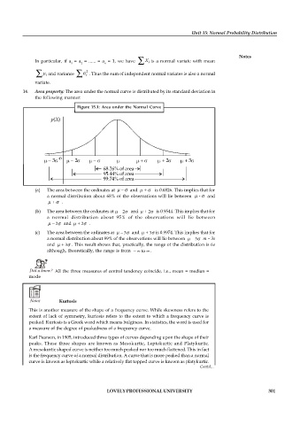
14. Area property: The area under the normal curve is distributed by its standard deviation in
the following manner:
Figure 15.1: Area under the Normal Curve

(a) The area between the ordinates at – and + is 0.6826. This implies that for
a normal distribution about 68% of the observations will lie between - and
+ .
(b) The area between the ordinates at – 2 and + 2 is 0.9544. This implies that for
a normal distribution about 95% of the observations will lie between
– 2 and + 2 .
(c) The area between the ordinates at – 3 and + 3 is 0.9974. This implies that for
a normal distribution about 99% of the observations will lie between – 3 m – 3s
and + 3 . This result shows that, practically, the range of the distribution is 6s
although, theoretically, the range is from – to .

Did u know? All the three measures of central tendency coincide, i.e., mean = median =
mode

Notes Kurtosis
This is another measure of the shape of a frequency curve. While skewness refers to the
extent of lack of symmetry, kurtosis refers to the extent to which a frequency curve is
peaked. Kurtosis is a Greek word which means bulginess. In statistics, the word is used for
a measure of the degree of peakedness of a frequency curve.
Karl Pearson, in 1905, introduced three types of curves depending upon the shape of their
peaks. These three shapes are known as Mesokurtic, Leptokurtic and Platykurtic.
A mesokurtic shaped curve is neither too much peaked nor too much flattened. This in fact
is the frequency curve of a normal distribution. A curve that is more peaked than a normal
curve is known as leptokurtic while a relatively flat topped curve is known as platykurtic.
Contd...

LOVELY PROFESSIONAL UNIVERSITY 301