Page 140 - DECO401_MICROECONOMIC_THEORY_ENGLISH

Unit-7: Recent Developments in Demand Theory

∆Q /Q Notes
because of which, b = x x
∆P /P
x x
where b is assumed to be constant.
By analysing Constant Elasticity of Demand Function of P , P and Y in form of multiple is presented as,
x Q
Log Q = log a + b log P + c log P + d log Y …(2)
x x o
To simplify e has not been taken from Equation (1),
ft
Converting Equation (2) into units, it becomes,
Q = a P P Y t …(3)
b
c
x x o
Graphic Presentation
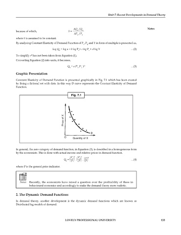
Constant Elasticity of Demand Function is presented graphically in Fig. 7.1 which has been created
by fixing a fictional set with data. In this way D curve represents the Constant Elasticity of Demand
Function.

Fig. 7.1

Price of X

D
O Quantity of X

In general, the zero category of demand function, in Equation (3), is described in a homogeneous form
by the economists. This is done with actual income and relative prices in demand function.
P b P c d
Y __
__
__

o

Q = ( ) . ( ) . ( ) …(4)

x

x P P P
where P is the general price indicator.
Recently, the economists have raised a question over the profitability of these in
behavioural economics and accordingly to make the demand theory more realistic.
2. The Dynamic Demand Functions
In demand theory, another development is the dynamic demand functions which are known as
Distributed lag models of demand.

LOVELY PROFESSIONAL UNIVERSITY 133