Page 186 - DECO402_Macro Economics

Unit-20: Effect of Monetary Policies Under Different Cases in IS-LM Framework

levels and actual GDP then we get the AD curve. Notes
The AD curve derived from IS-LM Equilibrium is
shown in figure 20.1

Notes The Aggregate Demand
Curve is found from the
joining of coincidences
of actual GDP and Price
level.

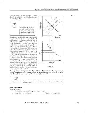
In figure 20.1 (A), the initial equilibrium in money
and product market is shown on point E where IS
curve intersects the LM curve. According to it, the
balanced actual GDP level is OY and interest rate
is Or. According to OY actual GDP the price level
is OP which is shown in part (B) of figure 20.1 by
point A. As there is a rise in price level, LM curve
becomes LM on being shifted. New equilibrium
1
point is E where IS curve cuts LM curve. According
1
to new equilibrium lower actual GDP is equal to OY
1
and higher interest rate is equal to Or . Lower GDP
1
(= OY ) and higher price level OP are shown by
1
1
point B in the part (B) in figure. With the reduction
in price level, LM curve becomes LM on being
2
shifted according to which higher actual GDP is
equal to OY and lower interest rate is equal to Or .
2
2
The coincidence of higher actual GDP (= OY ) and
2
lower price level OP is shown by point C in the
2
part (B) in figure. On joining A, B and C points, we
get the AD curve, which is downward sloped, and Figure 20.1
is inverse related with price level.
The slope of AD curve depends on the slopes of IS and LM curves which further depends on the
interest rate, the sensitivity of investment from the change in interest rate, coefficient multiplier
and the sensitivity of money demand from the change in actual GDP.

Did You Know? A new equilibrium is found from the lower level of GDP and higher level
of interest rate.

Self Assessment
Fill in the blanks:
1. On being money supply low, LM Curve shifts towards ....................
2. The IS-LM Model presents an .............................................. of derivation of A.D. curve.

LOVELY PROFESSIONAL UNIVERSITY 179