Page 184 - DECO503_INTERNATIONAL_TRADE_AND_FINANCE_ENGLISH

International Trade and Finance

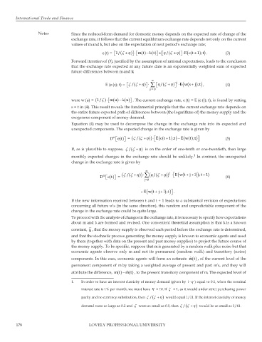
Notes Since the reduced-form demand for domestic money depends on the expected rate of change of the
exchange rate, it follows that the current equilibrium exchange rate depends not only on the current
values of m and k, but also on the expectation of next period’s exchange rate;
( ) k t−
e (t) = 1/ (ζ + η ) ⋅   mt ( ) +   η ( / ζ + η ) ⋅   E ( (e t + 1 ;t (3)


) ) .


 
Forward iteration of (3), justified by the assumption of rational expectations, leads to the conclusion
that the exchange rate expected at any future date is an exponentially weighted sum of expected
future differences between m and k;
∞
(
j
E (e (s); t) = ζ  / (ζ η+ ) ⋅  ∑  η  / (ζ η+ ) ⋅E ws ) ) , (4)

( + j
;t



j = 0
were w (u) = (1/ ζ )⋅ mu ( ) . The current exchange rate, e (t) = E (e (t); t), is found by setting
( ) − k u


s = t in (4). This result reveals the fundamental principle that the current exchange rate depends on
the entire future expected path of differences between (the logarithms of) the money supply and the
exogenous component of money demand.
Equation (4) may be used to decompose the change in the exchange rate into its expected and
unexpected components. The expected change in the exchange rate is given by
() = ( /ζ
) ) Et −
() )
D e et  (ζ η+ )) E et⋅   ( ( + 1 ; (w t ;t  (5)

If, as is plausible to suppose, ζ / (ζ η+ ) is on the order of one-tenth or one-twentieth, then large
1
monthly expected changes in the exchange rate should be unlikely. In contrast, the unexpected
change in the exchange rate is given by
∞ j 
( +
+
() =
D u et  (ζ / (ζ η+ )) ⋅ ∑ (η / (ζ η+ )) ⋅  E (wt j l )) ; t + 1) (6)

j=0
(
(
–E wt ++ ) )  .
j l
;t

If the new information received between t and t + 1 leads to a substantial revision of expectations
concerning all future w’s (in the same direction), this random and unpredictable component of the
change in the exchange rate could be quite large.
To proceed with the analysis of changes in the exchange rate, it is necessary to specify how expectations
about m and k are formed and revised. One convenient theoretical assumption is that k is a known
constant, k , that the money supply is observed each period before the exchange rate is determined,
and that the stochastic process generating the money supply is known to economic agents and used
by them (together with data on the present and past money supplies) to project the future course of
the money supply. To be specific, suppose that m is generated by a random walk plus noise but that
economic agents observe only m and not its permanent (random walk) and transitory (noise)
ˆ mt
components. In this case, economic agents will form an estimate ( ) , of the current level of the
permanent component of m by taking a weighted average of present and past m’s, and they will
()
attribute the difference, () − ˆ mt , to the present transitory component of m. The expected level of
mt
1. In order to have an interest elasticity of money demand (given by i η⋅ ) equal to 0.1, when the nominal
interest rate is 1% per month, we must have η = 10. If ζ = 1, as it would under strict purchasing power
parity and no currency substitution, then ζ / (ζ + η ) would equal 1/11. If the interest elasticity of money
demand were as large as 0.2 and ζ were as small as 0.5, then ζ / (ζ + η ) would be as small as 1/41.

178 LOVELY PROFESSIONAL UNIVERSITY