Page 96 - DMTH502_LINEAR_ALGEBRA

Linear Algebra

Notes 5.2 Row-reduced Echelon Matrices

Definition: An m × n matrix R is called a row-reduced echelon matrix if:
(a) R is row-reduced;

(b) every row of R which has all its entries 0 occurs below every row which has a non-zero entry;
(c) if rows 1,..., r are the non-zero rows of R, and if the leading non-zero entry of row i occurs
is column k , i = 1,..., r , then k < k < ... < k .
i 1 2 r
One can also describe an m × n row-reduced echelon matrix R as follows. Either every entry in R
is 0, or there exists a positive integer r, 1  r  m, and r positive integers k ,..., k with 1  k  n and
1 r i
(a) R = 0 for i > r, and R = 0 if j < k .
ij ij i
(b) R =  , 1  i  r, 1  j  r.
iki ij
(c) k < ... < k .
1 r

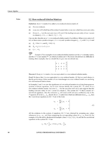
Example 4: Two examples of row-reduced echelon matrices are the n × n identity matrix,
and the m × n zero matrix 0 m, n , in which all entries are 0. The reader should have no difficulty in
making other examples, but we should like to give one non-trivial one:

 1 
 0 1  3 0 2 
 
 0 0 0 1 2 
 0 0 0 0 0 
 
 
Theorem 2: Every m × n matrix A is row-equivalent to a row-reduced echelon matrix.
Proof: We know that A is row-equivalent to a row-reduced matrix. All that we need observe is
that by performing a finite number of row interchanges on a row-reduced matrix we can bring
it to row-reduced echelon form.
In Examples 1 and 3, we saw the significance of row-reduced matrices in solving homogeneous
systems of linear equations. Let us now discuss briefly the system RX = 0, when R is a
row-reduced echelon matrix. Let rows 1,..., r be the non-zero rows of R, and suppose that the
leading non-zero entry of row i occurs in column k . The system RX = 0 then consists of r
i
non-trivial equations. Also the unknown x , will occur (with non-zero coefficient) only in the
k
i equation. If we let u ,...,u denote the (n – r) unknowns which are different from x ,...,x , then
th
1 n–r k1 kr
the r non-trivial equations in RX = 0 are of the form
n r 

x k 1   C u j  0 
1 j
j 1 
    ...(1)
n r 

x kr   C u j  0 
rj
j 1  
All the solutions to the system of equations RX = 0 are obtained by assigning any values
whatsoever to u ,...,u and then computing the corresponding values of x ,...,x from (1). For
1 n–r k1 kr
example, if R is the matrix displayed in Example 4, then r = 2, k = 2, k = 4, and the two non-trivial
1 2
equations in the system RX = 0 are
1 1
x – 3x + x = 0 or x = 3x – x
2 3 5 2 3 5
2 2
90 LOVELY PROFESSIONAL UNIVERSITY