Page 100 - DECO101_MICRO_ECONOMICS_ENGLISH

Unit 7: Production Theory

Notes
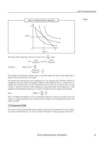
Figure 7.3: Optimum Factor Combination

Q 3
Q 2

Q 1

OA
The slope of the budget line or the isocost line will be – , where
OB
Cost Cost
OA = and OB =
Price of Y Price of X
OA
Therefore, Slope of AB = -
OB
Price of X P
= =- X
Price of Y P
Y
The negative sign indicates negative slope. In absolute terms, the slope of the budget line is
equal to the price ratio of the two inputs.

The budget line of the firm has been superimposed on its isoquant map. The firm would be in

equilibrium at a point where an isoquant is tangent to the budget line AB, i.e., point E. Thus in
equilibrium, the firm produces on the isoquant Q and uses OX units of input X and OY units

2
1
1
of input Y. At point E, the slope of the isoquant Q is equal to the slope of the budget line, i.e., the
2
marginal rate of technical substitution of X and Y is equal to the ratio of prices of two inputs.
MP P
Thus MRTS = MP X Y = P X Y
XY
Thus, to minimise production costs (or to maximise output for a given cost outlay), the extra
output or marginal product spent on labour must be equal to the marginal product per unit
spent on capital.
7.6 Expansion Path

The case of a firm producing 1000 units of output using 10 units of capital and 10 units of labour
(at point a) with input prices w=2 and r=2 is shown in Figure 7.4 using isoquants and isocosts.

LOVELY PROFESSIONAL UNIVERSITY 95