Page 314 - DCOM203_DMGT204_QUANTITATIVE_TECHNIQUES_I

Unit 15: Normal Probability Distribution

Table for the fitting of Normal Curve Notes
Class Mid-values X z N
z y z f *
e
Intervals (X) (from table)
10-20 15 2.34 0.0258 0.2081 2
20-30 25 1.53 0.1238 0.9984 10
30-40 35 0.73 0.3056 2.4645 25
40-50 45 0.08 0.3977 3.2073 32
50-60 55 0.89 0.2685 2.1653 22
60-70 65 1.69 0.0957 0.7718 8
70-80 75 2.50 0.0175 0.1411 1
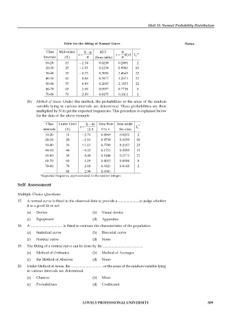
(b) Method of Areas: Under this method, the probabilities or the areas of the random
variable lying in various intervals are determined. These probabilities are then
multiplied by N to get the expected frequencies. This procedure is explained below
for the data of the above example.

Class Lower Limit X 44 Area from Area under *
z f
e
Intervals (X) 12.4 0 to z the class
10-20 10 2.74 0.4969 0.0231 2
20-30 20 1.94 0.4738 0.1030 10
30-40 30 1.13 0.3708 0.2453 25
40-50 40 0.32 0.1255 0.3099 31
50-60 50 0.48 0.1844 0.2171 22
60-70 60 1.29 0.4015 0.0806 8
70-80 70 2.10 0.4821 0.0160 2
80 2.90 0.4981
*Expected frequency approximated to the nearest integer.
Self Assessment

Multiple Choice Questions:
17. A normal curve is fitted to the observed data to provide a ........................to judge whether
it is a good fit or not

(a) Device (b) Visual device
(c) Equipment (d) Apparatus
18. A .................................... is fitted to estimate the characteristics of the population.
(a) Statistical curve (b) Binomial curve
(c) Normal curve (d) None
19. The fitting of a normal curve can be done by the .............................................
(a) Method of Ordinates (b) Method of Averages
(c) the Method of Abscissa (d) None

20. Under Method of Areas, the .................................... or the areas of the random variable lying
in various intervals are determined.
(a) Chances (b) Mean
(c) Probabilities (d) Coefficient

LOVELY PROFESSIONAL UNIVERSITY 309