Page 87 - DECO201_MACRO_ECONOMICS_ENGLISH

Macro Economics

Notes
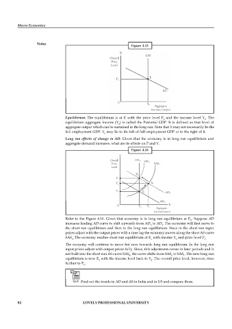
Figure 4.15

Equilibrium: The equilibrium is at E with the price level P and the income level Y . The
0 0
equilibrium aggregate income (Y ) is called the Potential GDP. It is defined as that level of
0
aggregate output which can be sustained in the long run. Note that it may not necessarily be the
full employment GDP. Y may lie to the left of full employment GDP or to the right of it.
0
Long run effects of change in AD: Given that the economy is in long run equilibrium and
aggregate demand increases, what are its effects on P and Y.

Figure 4.16

Refer to the Figure 4.16. Given that economy is in long run equilibrium at E . Suppose AD
0
increases leading AD curve to shift upwards from AD to AD . The economy will first move to
0 1
the short run equilibrium and then to the long run equilibrium. Since in the short run input
prices adjust with the output prices with a time lag the economy moves along the short AS curve
SAS . The economy reaches short run equilibrium at E with income Y and price level P .
0 1 1 1
The economy will continue to move but now towards long run equilibrium. In the long run
input prices adjust with output prices fully. Since, this adjustment comes in later periods and is
not built into the short run AS curve SAS , the curve shifts from SAS to SAS . The new long run
0 0 1
equilibrium is now E with the income level back to Y . The overall price level, however, rises
2 0
further to P .
2

Task Find out the trends in AD and AS in India and in US and compare them.

82 LOVELY PROFESSIONAL UNIVERSITY