Page 303 - DCOM303_DMGT504_OPERATION_RESEARCH

Operations Research

Notes
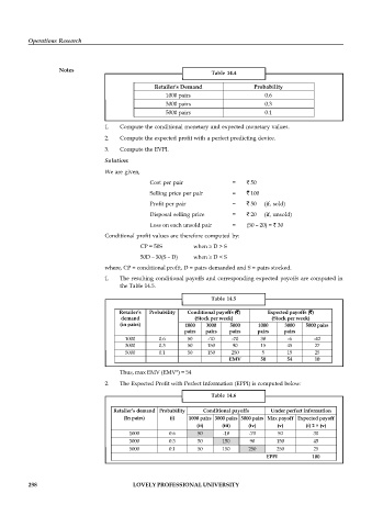
Table 14.4
Retailer's Demand Probability
1000 pairs 0.6
3000 pairs 0.3
5000 pairs 0.1

1. Compute the conditional monetary and expected monetary values.
2. Compute the expected profit with a perfect predicting device.
3. Compute the EVPI.

Solution:
We are given,
Cost per pair = ` 50
Selling price per pair = ` 100
Profit per pair = ` 50 (if, sold)
Disposal selling price = ` 20 (if, unsold)
Loss on each unsold pair = (50 – 20) = ` 30

Conditional profit values are therefore computed by:
CP = 50S when  D > S
50D – 30(S – D) when  D < S
where, CP = conditional profit, D = pairs demanded and S = pairs stocked.
1. The resulting conditional payoffs and corresponding expected payoffs are computed in
the Table 14.5.
Table 14.5

Retailer’s Probability Conditional payoffs (`) Expected payoffs (`)
demand (Stock per week) (Stock per week)
(in pairs) 1000 3000 5000 1000 3000 5000 pairs
pairs pairs pairs pairs pairs
1000 0.6 50 -10 -70 30 -6 -42
3000 0.3 50 150 90 15 45 27
5000 0.1 50 150 250 5 15 25
EMV 50 54 10

Thus, max EMV (EMV*) = 54
2. The Expected Profit with Perfect Information (EPPI) is computed below:
Table 14.6

Retailer’s demand Probability Conditional payoffs Under perfect information
(In pairs) (i) 1000 pairs 3000 pairs 5000 pairs Max payoff Expected payoff
(ii) (iii) (iv) (v) (i) 2 × (v)
1000 0.6 50 -10 -70 50 30
3000 0.3 50 150 90 150 45
5000 0.1 50 150 250 250 25
EPPI 100

298 LOVELY PROFESSIONAL UNIVERSITY