Page 227 - DMGT404 RESEARCH_METHODOLOGY

Unit 10: Time Series

Notes
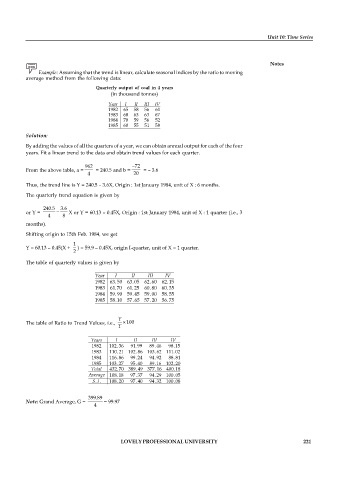
Example: Assuming that the trend is linear, calculate seasonal indices by the ratio to moving
average method from the following data:
Quarterly output of coal in 4 years
(in thousand tonnes)
Year I II III IV
1982 65 58 56 61
1983 68 63 63 67
1984 70 59 56 52
1985 60 55 51 58
Solution:

By adding the values of all the quarters of a year, we can obtain annual output for each of the four
years. Fit a linear trend to the data and obtain trend values for each quarter.

962  72
From the above table, a = = 240.5 and b = = – 3.6
4 20
Thus, the trend line is Y = 240.5 – 3.6X, Origin : 1st January 1984, unit of X : 6 months.
The quarterly trend equation is given by

240.5 3.6
or Y =  X or Y = 60.13 – 0.45X, Origin : 1st January 1984, unit of X : 1 quarter (i.e., 3
4 8
months).
Shifting origin to 15th Feb. 1984, we get
1
Y = 60.13 – 0.45(X + ) = 59.9 – 0.45X, origin I-quarter, unit of X = 1 quarter.
2
The table of quarterly values is given by

Year I II III IV
1982 63.50 63.05 62.60 62.15
1983 61.70 61.25 60.80 60.35
1984 59.90 59.45 59.00 58.55
1985 58.10 57.65 57.20 56.75

Y
The table of Ratio to Trend Values, i.e.,  100
T
Years I II III IV
1982 102.36 91.99 89.46 98.15
1983 110.21 102.86 103.62 111.02
1984 116.86 99.24 94.92 88.81
1985 103.27 95.40 89.16 102.20
Total 432.70 389.49 377.16 400.18
Average 108.18 97.37 94.29 100.05
S. I. 108.20 97.40 94.32 100.08

399.89
Note: Grand Average, G = = 99.97
4

LOVELY PROFESSIONAL UNIVERSITY 221