Page 89 - DCAP601_SIMULATION_AND_MODELING

Unit 6: Discrete System Simulation (III)

Notes
Example: Perhaps the simplest example of the method is its application to the evaluation
of the definite integral:
b
x
I   f ( )dx (1)
a
for the special case where f(x) >= 0. The value of I is the area under f(x) between x = a and x = b.
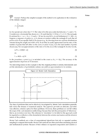
Consider now a horizontal line drawn at y = K such that f(x) <= K for a <= x<= b .The rectangle
R, enclosed by x = a, x = b, y = 0, and y = K has the area K( b– a) and furthermore I <= K(b – a).
Suppose a sequence of points (x , y ) is chosen at random within the rectangle R such that all
i i
points within R are equally likely to be chosen (e.g., by choosing from two uniform distributions
oriented along the length and width of R). It can then be easily appreciated that the ratio of the
number of points that fall either on the curve or under it (say, n) to the total number of points
chosen (say, N) is an approximation of the ratio of I to the area of the rectangle R. In other words,
n/N  I/[K(b – a)] (2)
Or
I  nK(b – a)/N (3)

In the procedure, a point (x ,y ) is included in the count n, if y <= f(x ). The accuracy of the
i i i i
approximation improves as N increases.
The interesting feature in this example is that the original problem is entirely deterministic and
yet the introduction of probabilistic notions can yield an approximation to its solution.

Figure 6.2: Monte Carlo Simulation

The class of problems that can be effectively investigated by Monte Carlo simulation generally
falls within the domain of numerical analysis. The approach provides an alternate, and often
very effective, solution option for these problems. However, these problems do not fall within
the scope of the and simulation methodology because they lack the prerequisite of ‘behaviour,’
that is, an evolution over time. The reference to ‘simulation’ in the label for the approach could
be regarded as a reflection of the dissimilarity between the solution mechanism and the inherent
nature of the problem.

Monte Carlo methods are a class of computational algorithms that rely on repeated random
sampling to compute their results. Monte Carlo methods are often used when simulating physical
and mathematical systems. Because of their reliance on repeated computation and random or

LOVELY PROFESSIONAL UNIVERSITY 83