Page 170 - DCAP605_ADVANCED_DATA_STRUCTURE_AND_ALGORITHMS

Unit 7: Splay Trees

Notes

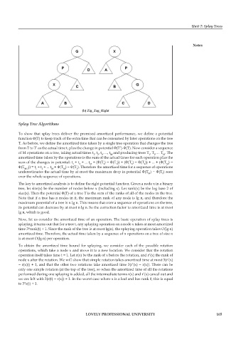
(b) Zig_Zag_Right

Splay Tree Algorithms

To show that splay trees deliver the promised amortized performance, we define a potential
function Φ(T) to keep track of the extra time that can be consumed by later operations on the tree
T. As before, we define the amortized time taken by a single tree operation that changes the tree

from T to T’ as the actual time t, plus the change in potential Φ(T’)-Φ(T). Now consider a sequence
of M operations on a tree, taking actual times t , t , t , ..., t and producing trees T , T , ... T . The
M
2
1
2
1
3
M
amortized time taken by the operations is the sum of the actual times for each operation plus the
sum of the changes in potential: t + t + ... t + (Φ(T ) − Φ(T )) + (Φ(T ) − Φ(T )) + ... + (Φ(T ) −
1 2 M 2 1 3 2 M
Φ(T M-1 )) = t + t + ... t + Φ(T ) − Φ(T ). Therefore the amortized time for a sequence of operations
1
2
1
M
M
underestimates the actual time by at most the maximum drop in potential Φ(T ) − Φ(T ) seen
1
M
over the whole sequence of operations.

The key to amortized analysis is to define the right potential function. Given a node x in a binary
tree, let size(x) be the number of nodes below x (including x). Let rank(x) be the log base 2 of
size(x). Then the potential Φ(T) of a tree T is the sum of the ranks of all of the nodes in the tree.
Note that if a tree has n nodes in it, the maximum rank of any node is lg n, and therefore the
maximum potential of a tree is n lg n. This means that over a sequence of operations on the tree,
its potential can decrease by at most n lg n. So the correction factor to amortized time is at most
lg n, which is good.
Now, let us consider the amortized time of an operation. The basic operation of splay trees is
splaying; it turns out that for a tree t, any splaying operation on a node x takes at most amortized
time 3*rank(t) + 1. Since the rank of the tree is at most lg(n), the splaying operation takes O(lg n)
amortized time. Therefore, the actual time taken by a sequence of n operations on a tree of size n
is at most O(lg n) per operation.
To obtain the amortized time bound for splaying, we consider each of the possible rotation
operations, which take a node x and move it to a new location. We consider that the rotation
operation itself takes time t = 1. Let r(x) be the rank of x before the rotation, and r’(x) the rank of
node x after the rotation. We will show that simple rotation takes amortized time at most 3(r’(x)
− r(x))) + 1, and that the other two rotations take amortized time 3(r’(x) − r(x)). There can be
only one simple rotation (at the top of the tree), so when the amortized time of all the rotations
performed during one splaying is added, all the intermediate terms r(x) and r’(x) cancel out and
we are left with 3(r(t) − r(x)) + 1. In the worst case where x is a leaf and has rank 0, this is equal
to 3*r(t) + 1.

LOVELY PROFESSIONAL UNIVERSITY 165