Page 154 - DECO101_MICRO_ECONOMICS_ENGLISH

Unit 10: Market Structure – Perfect Competition

This implies that at the minimum point of the LAC the corresponding (short run) plant is worked Notes
at its optimal capacity so that minimum of LAC and SAC coincide. On the other point, the LMC
cuts the LAC at its minimum point and the SMC cuts the SAC at its minimum.

Example: For a firm operating in a perfectly competitive market, the following data are

available
Price P = AR = MR = ` 20/- unit
Total cost function is C = 8 + 17Q – 4Q + Q 3
2
Let us find out the profit maximising output and the maximum profi t.

Marginal cost will be available if the first derivative of the total cost function is obtained. Thus,

d(C)
MC = = 17 – 8Q + 3Q 2
dQ
Maximum profit will be earned when

MC and MR are equal:
20 = 17 – 8Q + 3Q 2
Solving this equation gives two values for Q as –1/3 and 3. Obviously, negative output cannot be
produced; hence at Q = 3, the firm will maximise profits. Total revenue will be ` 60 and total cost

` 50. The maximum profit at the output of 3 units is ` 10.
Shut-down Decision
The supply curve of a competitive firm is its marginal curve. It is that part of the marginal cost

curve which is above the average variable cost curve.

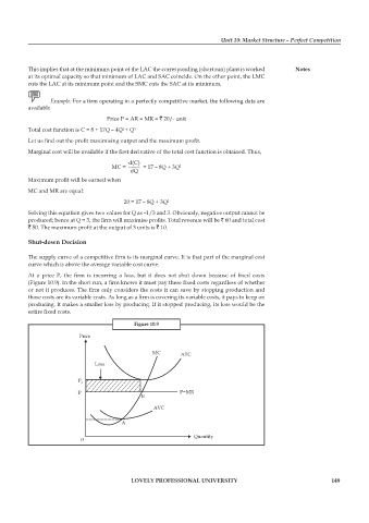
At a price P, the firm is incurring a loss, but it does not shut down because of fi xed costs
(Figure 10.9). In the short run, a firm knows it must pay these fixed costs regardless of whether

or not it produces. The firm only considers the costs it can save by stopping production and

those costs are its variable costs. As long as a firm is covering its variable costs, it pays to keep on
producing. It makes a smaller loss by producing. If it stopped producing, its loss would be the
entire fi xed costs.
Figure 10.9
Price

MC ATC

Loss

P 1
P P=MR
E
AVC

A
Quantity
0

LOVELY PROFESSIONAL UNIVERSITY 149