Page 191 - DCOM203_DMGT204_QUANTITATIVE_TECHNIQUES_I

Quantitative Techniques – I

Notes equation then it implies that Y is exactly equal to 20 when X = 5. However, if Y = 10 + 2X is a
regression equation, then Y = 20 is an average value of Y when X = 5.

The term regression was first introduced by Sir Francis Galton in 1877.
Did u know?

9.1 Two Lines of Regression

For a bivariate data (X , Y ), i = 1,2, ...... n, we can have either X or Y as independent variable. If X
i i
is independent variable then we can estimate the average values of Y for a given value of X. The
relation used for such estimation is called regression of Y on X. If on the other hand Y is used for
estimating the average values of X, the relation will be called regression of X on Y. For a
bivariate data, there will always be two lines of regression. It will be shown later that these two
lines are different, i.e., one cannot be derived from the other by mere transfer of terms, because
the derivation of each line is dependent on a different set of assumptions.

9.1.1 Line of Regression of Y on X

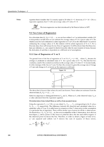
The general form of the line of regression of Y on X is Y = a + bX , where Y denotes the
Ci i Ci
average or predicted or calculated value of Y for a given value of X = X . This line has two
i
constants, a and b. The constant a is defined as the average value of Y when X = 0. Geometrically,
it is the intercept of the line on Y-axis. Further, the constant b, gives the average rate of change
of Y per unit change in X, is known as the regression coefficient.
Figure 9.1

The above line is known if the values of a and b are known. These values are estimated from the
observed data (X , Y ), i = 1,2, ...... n.
i i
Note: It is important to distinguish between Y and Y . Where as Y is the observed value, Y is
Ci i i Ci
a value calculated from the regression equation.
Deviation taken from Actual Mean as well as from assumed mean
Using the regression Y = a + bX , we can obtain Y , Y , ...... Y corresponding to the X values
Ci i C1 C2 Cn
X , X , ...... X respectively. The difference between the observed and calculated value for a
1 2 n
th
particular value of X say X is called error in estimation of the i observation on the assumption
i
of a particular line of regression. There will be similar type of errors for all the n observations.
We denote by e = Y - Y (i = 1,2,.....n), the error in estimation of the i observation. As is obvious
th
i i Ci
from figure, e will be positive if the observed point lies above the line and will be negative if
i
the observed point lies below the line. Therefore, in order to obtain a figure of total error,
s
e ' are squared and added. Let S denote the sum of squares of these errors,
i
n n
S e 2 Y Y 2
i.e., i i Ci .
i 1 i 1
186 LOVELY PROFESSIONAL UNIVERSITY