Page 274 - DCOM203_DMGT204_QUANTITATIVE_TECHNIQUES_I

Unit 13: Binomial Probability Distribution

The set of all possible values of the random variable X along with their respective probabilities Notes
is termed as Probability Distribution of X. The probability distribution of X, defined in example
above, can be written in a tabular form as given below:
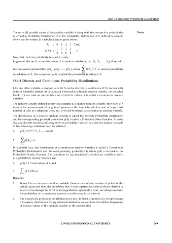
X : 0 1 2 3 Total
1 3 3 1
p X : 1
8 8 8 8
Note that the total probability is equal to unity.
In general, the set of n possible values of a random variable X, i.e., {X , X , ...... X } along with
1 2 n
n
their respective probabilities p(X ), p(X ), ...... p(X ), where p X 1, is called a probability
1 2 n i
i 1
distribution of X. The expression p(X) is called the probability function of X.
13.1.2 Discrete and Continuous Probability Distributions

Like any other variable, a random variable X can be discrete or continuous. If X can take only
finite or countably infinite set of values, it is termed as a discrete random variable. On the other
hand, if X can take an uncountable set of infinite values, it is called a continuous random
variable.
The random variable defined in previous example is a discrete random variable. However, if X
denotes the measurement of heights of persons or the time interval of arrival of a specified
number of calls at a telephone desk, etc., it would be termed as a continuous random variable.
The distribution of a discrete random variable is called the Discrete Probability Distribution
and the corresponding probability function p(X) is called a Probability Mass Function. In order
that any discrete function p(X) may serve as probability function of a discrete random variable
X, the following conditions must be satisfied:
1. p(X ) 0 i = 1, 2, ...... n and
i
n
2. p X i 1
i 1
In a similar way, the distribution of a continuous random variable is called a Continuous
Probability Distribution and the corresponding probability function p(X) is termed as the
Probability Density Function. The conditions for any function of a continuous variable to serve
as a probability density function are:
1. p(X) 0 real values of X, and

2. p X dX 1

Remarks:
1. When X is a continuous random variable, there are an infinite number of points in the
sample space and thus, the probability that X takes a particular value is always defined to
be zero even though the event is not regarded as impossible. Hence, we always measure
the probability of a continuous random variable lying in an interval.

2. The concept of a probability distribution is not new. In fact it is another way of representing
a frequency distribution. Using statistical definition, we can treat the relative frequencies
of various values of the random variable as the probabilities.

LOVELY PROFESSIONAL UNIVERSITY 269