Page 309 - DCOM203_DMGT204_QUANTITATIVE_TECHNIQUES_I
P. 309
Quantitative Techniques – I


                    Notes
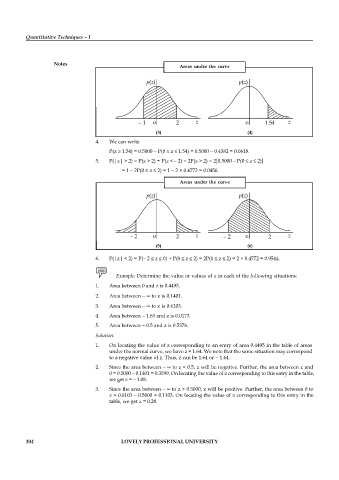
                                                                Areas  under  the  curve


                                                        (3)                                                                  (4)
                                   4.  We can write
                                       P(z   1.54) = 0.5000   P(0   z   1.54) = 0.5000   0.4382 = 0.0618.
                                   5.  P(|z| > 2) = P(z > 2) + P(z <   2) = 2P(z > 2) = 2[0.5000   P(0   z   2)]
                                                 = 1   2P(0   z   2) = 1   2 × 0.4772 = 0.0456.

                                                                Areas  under  the  curve


                                                        (5)                                                                  (6)
                                   6.  P(|z| < 2) = P(  2   z   0) + P(    z   2) = 2P(    z   2) = 2 × 0.4772 = 0.9544.


                                          Example: Determine the value or values of z in each of the following situations:
                                   1.  Area between 0 and z is 0.4495.
                                   2.  Area between    to z is 0.1401.

                                   3.  Area between    to z is 0.6103.
                                   4.  Area between   1.65 and z is 0.0173.
                                   5.  Area between   0.5 and z is 0.5376.
                                   Solution:
                                   1.  On locating the value of z corresponding to an entry of area 0.4495 in the table of areas
                                       under the normal curve, we have z = 1.64. We note that the same situation may correspond
                                       to a negative value of z. Thus, z can be 1.64 or   1.64.
                                   2.  Since the area between    to z < 0.5, z will be negative. Further, the area between z and
                                       0 = 0.5000   0.1401 = 0.3599. On locating the value of z corresponding to this entry in the table,
                                       we get z =   1.08.
                                   3.  Since the area between    to z > 0.5000, z will be positive. Further, the area between 0 to
                                       z = 0.6103   0.5000 = 0.1103. On locating the value of z corresponding to this entry in the
                                       table, we get z = 0.28.


          304                               LOVELY PROFESSIONAL UNIVERSITY

