Page 31 - DCOM203_DMGT204_QUANTITATIVE_TECHNIQUES_I

Quantitative Techniques – I

Notes This frequency distribution does not reveal any pattern of behaviour of the variable. In
order to bring the behaviour of the variable into focus, it becomes necessary to convert
this into a grouped frequency distribution.
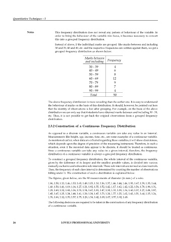
Instead of above, if the individual marks are grouped like marks between and including
30 and 39, 40 and 49, etc. and the respective frequencies are written against them, we get a
grouped frequency distribution as shown below:

30 - 39 4
40 - 49 6
50 - 59 8
60 - 69 12
70 - 79 9
80 - 89 7
90 - 99 4
50

The above frequency distribution is more revealing than the earlier one. It is easy to understand
the behaviour of marks on the basis of this distribution. It should, however, be pointed out here
that the identity of observations is lost after grouping. For example, on the basis of the above
distribution we can only say that 4 students have obtained marks between and including 30 - 39,
etc. Thus, it is not possible to get back the original observations from a grouped frequency
distribution.

2.3.2 Construction of a Continuous Frequency Distribution

As opposed to a discrete variable, a continuous variable can take any value in an interval.
Measurements like height, age, income, time, etc., are some examples of a continuous variable.
As mentioned earlier, when data are collected regarding these variables, it will show discreteness,
which depends upon the degree of precision of the measuring instrument. Therefore, in such a
situation, even if the recorded data appear to be discrete, it should be treated as continuous.
Since a continuous variable can take any value in a given interval, therefore, the frequency
distribution of a continuous variable is always a grouped frequency distribution.

To construct a grouped frequency distribution, the whole interval of the continuous variable,
given by the difference of its largest and the smallest possible values, is divided into various
mutually exclusive and exhaustive sub-intervals. These sub-intervals are termed as class intervals.
Then, the frequency of each class interval is determined by counting the number of observations
falling under it. The construction of such a distribution is explained below:
The figures, given below, are the 90 measurements of diameter (in mm.) of a wire.
1.86, 1.58, 1.13, 1.46, 1.53, 1.65, 1.49, 1.03, 1.10, 1.36, 1.37, 1.46, 1.44, 1.46, 1.95, 1.67, 1.59, 1.35, 1.44,
1.40, 1.50, 1.41, 1.19, 1.16, 1.27, 1.21, 1.82, 1.55, 1.52, 1.42, 1.17, 1.62, 1.42, 1.22, 1.56, 1.78, 1.98, 1.31,
1.29, 1.69, 1.32, 1.68, 1.36, 1.55, 1.54, 1.67, 1.81, 1.47, 1.30, 1.33, 1.38, 1.34, 1.40, 1.37, 1.27, 1.04, 1.87,
1.45, 1.47, 1.35, 1.24, 1.48, 1.41, 1.39, 1.38, 1.47, 1.73, 1.20, 1.77, 1.25, 1.62, 1.43, 1.51, 1.60, 1.15, 1.26,
1.76, 1.66, 1.12, 1.70, 1.57, 1.75, 1.28, 1.56, 1.42, 1.09, 1.07, 1.57, 1.92, 1.48.

The following decisions are required to be taken in the construction of any frequency distribution
of a continuous variable.

26 LOVELY PROFESSIONAL UNIVERSITY