Page 72 - DECO201_MACRO_ECONOMICS_ENGLISH
P. 72
Unit 4: Theories of Income, Output and Employment: Keynesian Theory


          Therefore,    S = Y - (a + bY)                                                        Notes
                          = Y - a - bY
                          = -a + (1 - b) Y
          where        - a = saving at zero income

                    (1 - b) = the proportion of increase in income saved.

               !
             Caution  In the function, -a is constant. (1-b) equals change in saving (S) divided by change
             in income (Y). It is also called Marginal Propensity to Save (MPS).
                    S
             1– b      MPS
                    Y

                                            Figure  4.4


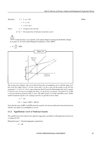
          The saving curve (Figure 4.4) can be derived from the consumption curve with the help of 45  º
                                                                                   º
          line from the origin. Given Y on the x-axis and C on the y-axis, all the points on the 45 line
                                                     º
          represent C = Y or S = O. The C curve intersects the 45 line at B which means that at B, Y equals
          C and S is zero. To derive a straight line curve, we need only two points. One point is B  on the
                                                                                1
          x-axis derived from point B on the C curve. The other point, is S on the extended y-axis. At this
          point OS must be equal to OC. Joining S and B1, we get the S curve. Here:
                       -a = OS

                      1-b = slope = MPS =  S/ Y
          Note that the sum of MPC and MPS must be equal to one because that part of increased income
          which is not spent on consumption is saved.
          4.1.2  Equilibrium Level of National Income


          The equilibrium is determined where planned aggregate expenditure (AE) equals planned income
          or output (Y) AE.

          Planned income = Planned aggregate expenditure.
                      Y = AE


                                           LOVELY PROFESSIONAL UNIVERSITY                                   67

