Page 86 - DECO201_MACRO_ECONOMICS_ENGLISH

Unit 4: Theories of Income, Output and Employment: Keynesian Theory

Notes
Example: One such example is change in oil prices. A rise in oil price shift SRAS curve to the
left. Such cost changes are called cost stocks or supply stocks.
Economic Growth: Aggregate supply curve is based on the assumption that resources are
fixed. But when economic growth takes place resources increase. This causes rightward
shift of the SAS curve.
Decrease in Resources: Resources may decrease due to many reasons, economic or
non-economic. One economic reason is deterioration and wearing out of capital if not
properly maintained. If it is not replaced by new capital, the stock of capital will decrease.
This will shift the SAS curve to the left.
Non-economic factors like bad weather, wars, natural disasters, etc. destroy resources and
lead to the leftward shift of the SAS curve.

Government Policies: Governments do take policy measures to increase incentives to
work and invest. For example, policy measures taken in India recently aimed at
liberalization, privatization and globalization. Some examples are reduction in taxes,
delicensing, removing trade barriers, etc. These shift the SAS curve to the right.

Equilibrium Overall Price Level

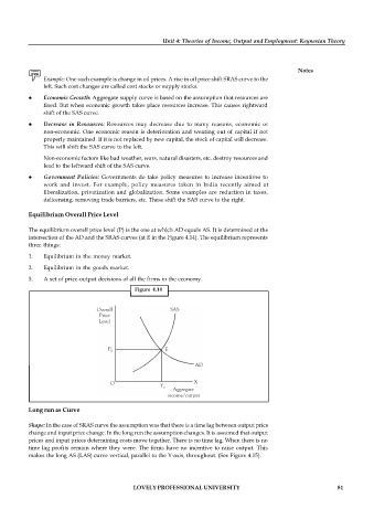
The equilibrium overall price level (P) is the one at which AD equals AS. It is determined at the
intersection of the AD and the SRAS curves (at E in the Figure 4.14). The equilibrium represents
three things:
1. Equilibrium in the money market.

2. Equilibrium in the goods market.
3. A set of price-output decisions of all the firms in the economy.
Figure 4.14

Long run as Curve

Shape: In the case of SRAS curve the assumption was that there is a time lag between output price
change and input price change. In the long run the assumption changes. It is assumed that output
prices and input prices determining costs move together. There is no time lag. When there is no
time lag profits remain where they were. The firms have no incentive to raise output. This
makes the long AS (LAS) curve vertical, parallel to the Y-axis, throughout. (See Figure 4.15).

LOVELY PROFESSIONAL UNIVERSITY 81