Page 99 - DECO201_MACRO_ECONOMICS_ENGLISH

Macro Economics

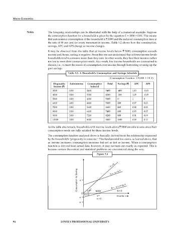
Notes The foregoing relationships can be illustrated with the help of a numerical example. Suppose
the consumption function for a household is given by the equation C = 1000 + 0.8Y. This means
that autonomous consumption of the household is 1000 and the induced consumption rises at
the rate of 80 per cent for every increment in income. Table 5.2 shows how the consumption,
savings, APC and APS change as income changes.
It may be observed from the table that at income levels below 5000, consumption exceeds
income and, hence, saving is negative. From this one can understand that at lower income levels
households tend to consume more than they earn. In other words, they find their incomes rather
too low to meet their consumption needs. As a result, low income households are constrained to
dissave, i.e., to meet the excess of consumption over income through borrowing or using up the
past savings.

Table 5.2: A Household's Consumption and Savings Schedule
(Consumption Function: C=1000 + 0.8 Y)
Disposable Autonomous Consumption Total Savings ( ) APC APS
Income ( ) Induced
3000 1000 2400 3400 -400 1.13 -0.13
4000 1000 3200 4200 -200 1.05 -0.05
5000 1000 4000 5000 0 1 0
6000 1000 4800 5800 200 0.97 0.03
7000 1000 5600 6600 400 0.94 0.06
8000 1000 6400 7400 600 0.93 0.07
9000 1000 7200 8200 800 0.91 0.09
10000 1000 8000 9000 1000 0.90 0.10

As the table also reveals, households with income levels above 5000 are able to save since their
consumption needs are fully satisfied by these income levels.

The consumption function analysed above is basically derived from the relationship expressed
by the household's "propensity to consume". This fundamental law states, as learned above, that
as income increases, consumption increases but not as fast as income. When a consumption
function is derived from actual data, however, it may not turn out exactly as expected. This is
because various theoretical and statistical problems are encountered along the way.
Figure 5.4

94 LOVELY PROFESSIONAL UNIVERSITY