Page 275 - DCOM203_DMGT204_QUANTITATIVE_TECHNIQUES_I

Quantitative Techniques – I

Notes
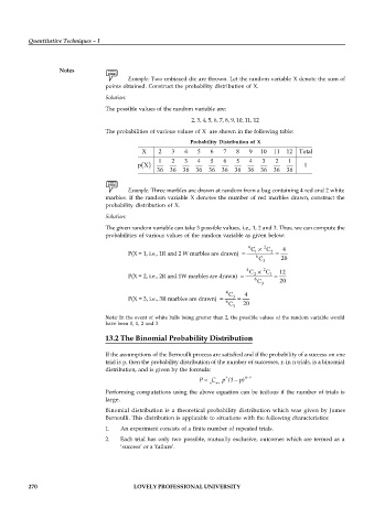
Example: Two unbiased die are thrown. Let the random variable X denote the sum of
points obtained. Construct the probability distribution of X.
Solution:
The possible values of the random variable are:
2, 3, 4, 5, 6, 7, 8, 9, 10, 11, 12

The probabilities of various values of X are shown in the following table:
Probability Distribution of X
X 2 3 4 5 6 7 8 9 10 11 12 Total
1 2 3 4 5 6 5 4 3 2 1
p X 1
36 36 36 36 36 36 36 36 36 36 36

Example: Three marbles are drawn at random from a bag containing 4 red and 2 white
marbles. If the random variable X denotes the number of red marbles drawn, construct the
probability distribution of X.

Solution:
The given random variable can take 3 possible values, i.e., 1, 2 and 3. Thus, we can compute the
probabilities of various values of the random variable as given below:

4 2
C C 4
P(X = 1, i.e., 1R and 2 W marbles are drawn) 1 2
6
C 3 20
4 2
C C 12
P(X = 2, i.e., 2R and 1W marbles are drawn) 2 1
6
C 3 20
4
C 4
P(X = 3, i.e., 3R marbles are drawn) 3
6
C 3 20
Note: In the event of white balls being greater than 2, the possible values of the random variable would
have been 0, 1, 2 and 3.
13.2 The Binomial Probability Distribution

If the assumptions of the Bernoulli process are satisfied and if the probability of a success on one
trial is p, then the probability distribution of the number of successes, r, in n trials, is a binomial
distribution, and is given by the formula:

Performing computations using the above equation can be tedious if the number of trials is
large.
Binomial distribution is a theoretical probability distribution which was given by James
Bernoulli. This distribution is applicable to situations with the following characteristics:
1. An experiment consists of a finite number of repeated trials.
2. Each trial has only two possible, mutually exclusive, outcomes which are termed as a
‘success’ or a ‘failure’.

270 LOVELY PROFESSIONAL UNIVERSITY