Page 276 - DCOM203_DMGT204_QUANTITATIVE_TECHNIQUES_I

Unit 13: Binomial Probability Distribution

3. The probability of a success, denoted by p, is known and remains constant from trial to Notes
trial. The probability of a failure, denoted by q, is equal to 1 – p.
4. The sequence of trials under the above assumptions is also termed as Bernoulli Trials

!
Caution Different trials are independent, i.e., outcome of any trial or sequence of trials has
no effect on the outcome of the subsequent trials.

13.2.1 Probability Function or Probability Mass Function

Let n be the total number of repeated trials, p be the probability of a success in a trial and q be the
probability of its failure so that q = 1 – p.
Let r be a random variable which denotes the number of successes in n trials. The
possible values of r are 0, 1, 2, ...... n. We are interested in finding the probability of r successes
out of n trials, i.e., P(r).

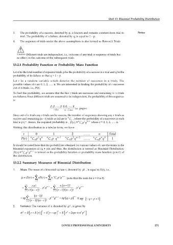
To find this probability, we assume that the first r trials are successes and remaining n – r trials
are failures. Since different trials are assumed to be independent, the probability of this sequence
is

.
p q q. ....
p p. ....
.
q
      i.e. prqn-r.




r times n r times

Since out of n trials any r trials can be success, the number of sequences showing any r trials as
n
success and remaining (n – r) trials as failure is C , where the probability of r successes in each
r
n
r n- r
r n-r
trial is p q . Hence, the required probability is , P(r) = C p q where r = 0, 1, 2, ...... n.
r
Writing this distribution in a tabular form, we have:
0 1 2 
( ) 0 0 1 1 2 2 2  0 1
It should be noted here that the probabilities obtained for various values of r are the terms in the
binomial expansion of (q + p)n and thus, the distribution is termed as Binomial Distribution.
n r n- r
P(r) = C p q is termed as the probability function or probability mass function (p.m.f.) of
r
the distribution.
13.2.2 Summary Measures of Binomial Distribution
1. Mean: The mean of a binomial variate r, denoted by , is equal to E(r), i.e.,
n n
n
r
r
r
E ( ) rP ( ) . r C p q n r (note that the term for r = 0 is 0)
r
r 0 r 1
n r . ! n . n n 1 !
n
r
r
. p q n r . p q n r
! r n r ! r 1 ! n r !
r 1 r 1
n n 1 ! n 1
1 n r
r
np . p q np q p = np  q p 1
1 r 1 ! n r !
r
2. Variance: The variance of r, denoted by 2 , is given by
2 2 2 2 2 2
E r E r E r np E r 2npr n p
LOVELY PROFESSIONAL UNIVERSITY 271