Page 74 - DECO401_MICROECONOMIC_THEORY_ENGLISH

Unit-4: Ordinal Utility Theory: Indifference Curve Approach

more than negative income effect. So the demand is less when price increases and the theory Notes
of demand is also implemented in inferior goods.
Price Effect = SQ; Substitution Effect = TQ; Income Effect = –TS

Then SQ (Price Effect) = TQ (Substitution Effect) + (–) TS (Income Effect) = SQ
(b) Substitution Effect and Income Effect for Inferior Goods in case of Price Fall: The separation
of substitution effect and income effect for inferior goods due to price fall can be described as
follows:

To Remember
The substitution effect always displays the consumption of cheap goods rather than costly goods. No matter that goods
are normal or inferior. So we do not put (+) or (–) prior to substitution effect.

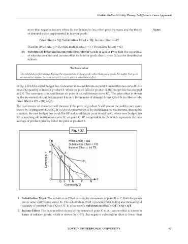
In Fig. 4.27 LM is initial budget line. Consumer is in equilibrium on point B on indifference curve IC. He
buys OQ quantity of inferior product X. When the price falls for product X, the budget line has slopped
as LN. The consumer is in equilibrium on point A on indifference curve IC . The price effect is shown
1
by the movement of equilibrium point B to A or the increase of demand from OQ to OS. In other words,
Price Effect = OS – OQ = QS.
The real income of consumer will increase if the price of product X will rise as the indifference curve
shows by sloping from IC to IC . If we stood consumer on IC by stablalizing his real income, then in this
1
situation, the new budget line would be RP and equilibrium point would be C, where new budget line
RP is touching old indifference curve IC on point C. RP is equivalent to LN which represents the new
average of product price by fall of the price of product X.

Fig. 4.27

Y Price Effect = SQ
L Substitution Effect = TQ
Income Effect = (–) TS
R
Commodity Y B C IC 1
A

IC
O X
QS TM P N
Commodity X

1. Substitution Effect: The substitution Effect is rising by movement of point B to C. Both the points
are in same indifference curve IC. The substitution effect represents price falling and increasing of
quantity of product from OQ to OT. In other words, substitution effect = OT – OQ = QT.
2. Income Effect: The income effect shown by movement of point C to A. Income effect is lowest in
terms of inferior goods, which is shown by (–ST). But negative substitution effect is lower than

LOVELY PROFESSIONAL UNIVERSITY 67