Page 81 - DECO401_MICROECONOMIC_THEORY_ENGLISH

Microeconomic Theory

Notes In the word of Lipsey, “Every point on the Price Consumption Curve corresponds to both the price of
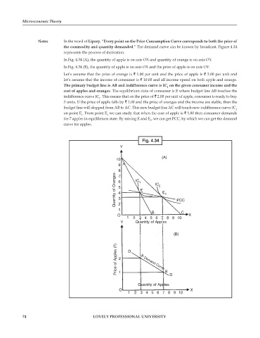
the commodity and quantity demanded.” The demand curve can be known by broadcast. Figure 4.34
represents the process of derivation.

In Fig. 4.34 (A), the quantity of apple is on axis OX and quantity of orange is on axis OY.
In Fig. 4.34 (B), the quantity of apple is on axis OX and the price of apple is on axis OY.
Let’s assume that the price of orange is 1.00 per unit and the price of apple is 2.00 per unit and
let’s assume that the income of consumer is 10.00 and all income spend on both apple and orange.
The primary budget line is AB and indifference curve is IC on the given consumer income and the
1
cost of apples and oranges. The equilibrium state of consumer is E where budget line AB touches the
indifference curve IC . This means that on the price of 2.00 per unit of apple, consumer is ready to buy
1
3 units. If the price of apple falls by 1.00 and the price of oranges and the income are stable, then the
budget line will slopped from AB to AC. This new budget line AC will touch new indifference curve IC
2
on point E . From point E we can study that when the cost of apple is 1.00 then consumer demands
1
1
for 7 apples in equilibrium state. By mixing E and E , we can get PCC, by which we can get the demand
1
curve for apples.
Fig. 4.34
Y

(A)
10
9 A
8
Quantity of Oranges 6 IC 1 E IC 2 E 1
7
5
4
3
2
1 PCC
B C
O X
1 23 456789 10
Y Quantity of Apples

(B)

Price of Apples (`) 2 D A Demand Curve B

1

Quantity of Apples D
O X
1 2 3456789 10

74 LOVELY PROFESSIONAL UNIVERSITY