Page 82 - DECO402_Macro Economics

Unit-9: Permanent Income and Life Cycle Hypothesis

Where Y = permanent income in current period, Y = Current income in current period, Y = the Notes
t
pt
t–1
previous period’s income; a = the ratio of change in income between previous period (t – 1) and present
period. This equation tells that the permanent income is the sum of income of current period (Yt) and
previous period’s income (Y ) and the ratio of income change in both (a). If current income sudden
t–1
increases then there will be less increase in permanent income. For increasing the permanent income,
we’ve to increase the income till many years continuously. Then people will think it as increased.
From the combination of equation (4) and (5), the short-termed and long-termed consumption function
can be expressed as following:
Ct = KY = K a Y + K (1 – a) Y ...(6)
t–1
t
pt
Where C = the consumption of current period, ka = short-termed MPC; k = long-termed MPC; and
t
(1 – a) Y is the intercept of short-termed consumption function.
t–1
According to Friedman, k and ka are different from each other and k >ka. Then k is equal to 1
approximately and ka is equals to 0 (zero).
Equation (6) tells that consumption depends on previous and current income both. Previous income
is so important for consumption that it is helpful to people in future forecasting of income.

Notes Current or measured income determines the consumption expenditure.

Its Assumptions: Friedman has presented the following assumptions about constant and variable
parts of income and consumption –
1. There is no any correlation between variable and constant income.
2. There is no any correlation between variable and constant consumption.
3. There is no any correlation between variable consumption and variable income.
4. Only the changes in constant income affect the consumption in organized form.
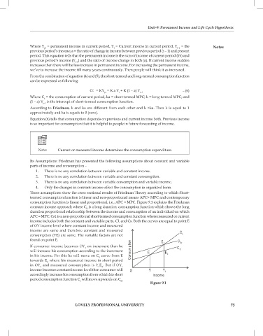
These assumptions show the cross sectional results of Friedman Theory according to which Short-
termed consumption function is linear and non-proportional means APC> MPC and contemporary
consumption function is linear and proportional, i.e., APC = MPC. Figure 9.1 explains the Friedman
constant income approach where C is a long duration consumption function which shows the long
L
duration proportional relationship between the income and consumption of an individual on which
APC = MPC. Cs1 is a non-proportional short termed consumption function where measured or current
income includes both the constant and variable parts, CL and Cs. Both the curves are equal to point E
of OY income level where constant income and measured
income are same and therefore constant and measured
consumption (YE) are same. The variable factors are not
found on point E.
If consumer income becomes OY on increment then he
1
will increase his consumption according to the increment
in his income. For this he will move on C curve from E
S
towards E where his measured income in short period
2
in OY and measured consumption is Y E . But if OY
1
1
1
2
income becomes constant income level then consumer will
accordingly increase his consumption from which his short
period consumption function C will move upwards on C
s
S1
Figure 9.1
LOVELY PROFESSIONAL UNIVERSITY 75