Page 324 - DECO504_STATISTICAL_METHODS_IN_ECONOMICS_ENGLISH
P. 324
Unit 25 : Methods of Moving Averages


                total is obtained by dropping the value of the first period from, and adding the value of the  Notes
                thirteenth period to the first moving total, and so on until all the moving total have been obtained
                from the series. Then each moving total is divided by 12 to get the 12-period moving averages.
                The moving totals and moving averages so obtained fall in between two periods. However,
                data that are typical of a period should be centred at the middle of the period. Thus, to compute
                moving averages when an even number of time units is used, an additional step is required to
                centre the averages at the middle of each time unit. For a 12-period moving average, centred
                averages are obtained by adding the two averages at a time and dividing each sum by 2. Thus,
                the first centred 12-period moving average would fall on the seventh period of the series, the
                second on the eighth period, and so on.
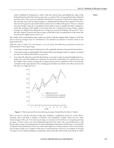
            The results of the computations made earlier are plotted with the original data in Figure 1. Both the
            sets of moving averages may be considered as the statistical expression of secular trend of our
            hypothetical data.
            With the help of Table 25.1 and Figure 1, we can make the following conclusions about the
            characteristics of moving average :
            1.  A moving average of equal length period will completely eliminate the periodic fluctuations.
            2.  A moving average of equal length will be linear if the series changes on the average by a constant
                per time unit and its fluctuations are periodic.
            3.  Even when the data show periodic fluctuations, a moving average of unequal length period, no
                matter how small the difference is between the duration of periodicity of original series, and
                the length of the moving average, the moving average cannot completely remove the periodic
                variations in the original series. The averaging process then only tends to smooth out somewhat
                the short-run highs and lows.

                             8.0

                             7.0

                             6.0

                             5.0

                             4.0

                             3.0
                                                  ORIGINAL DATA
                                                  3-YEAR MOVING AVERAGE
                             2.0                  5-YEAR MOVING AVERAGE

                             1.0

                               0
                                   1   3   5   7  9   11  13  15  17  19 20
                                                 YEAR
                 Figure 1 : Three-year and Five-year Moving Average Trends Fitted to Data in Table 1
            Thus, we can see that the moving average may constitute a satisfactory trend for a series that is
            basically linear and that is regular in duration and amplitude. Further, there are two other
            disadvantages in the use of the moving average as a measure of trend. First, in computing moving
            averages, we loose some years at the beginning and end of the series. The second drawback is that
            the moving average is not represented by some mathematical formulae and, therefore, is not capable
            of objective future projections. Since one of the major objectives of trend analysis is that of forecasting,
            the moving average is no longer in wide use as a trend measure. However, the method of moving
            averages is a very useful technique in analyzing a time series data. First of all, in problems in which


                                             LOVELY PROFESSIONAL UNIVERSITY                                      319

