Page 195 - DMTH504_DIFFERENTIAL_AND_INTEGRAL_EQUATION

Differential and Integral Equation

Notes 11.4 Bessel’s Inequality, Approximation in the Mean and
Completeness

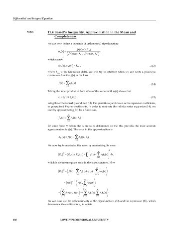
We can now define a sequence of orthonormal eigenfunctions
y
x
r ( ) ( , n )
x
x
( )
n
y
r ( ) ( , n ), r ( ) ( , n )
x
y
x
x
x
which satisfy
x
( ), ( ) nm , ...(13)
x
n m
where is the Kronecker delta. We will try to establish when we can write a piecewise
nm
continuous function f(x) in the form

x
x
f ( ) a f ( ) ...(14)
i i
i 0
Taking the inner product of both sides of this series with (x) shows that
j
a j f ( ), j ( ) , ...(15)
x
x
using the orthonormality condition (13). The quantities a are known as the expansion coefficients,
i
or generalized Fourier coefficients. In order to motivate the infinite series expansion (14), we
start by approximating f(x) by a finite sum,
Ν
x
x
f ( ) A f ( , )
N i i
i 0
for some finite N, where the A are to be determined so that this provides the most accurate
i
approximation to f(x). The error in this approximation is
Ν
x
x
R N ( ) f ( ) A f ( , i )
x
i
i 0
We now try to minimize this error by minimizing its norm
2
b Ν
2
x
x
x
x
R N R N ( ), R N ( ) f ( ) A f ( ) dx ,
i i
a
i 0
which is the mean square error in the approximation. Now
Ν Ν
2
x
f
x
x
x
R N f ( ) A f ( ), ( ) A f ( )
i i
i i
i 0 i 0
Ν
2
x
x
f ( ) f ( ), A f ( )
x
i i
i 0
Ν Ν Ν
x
f
A f ( ), ( ) A f ( ), A f ( )
x
x
x
i i
i i
i i
i 0 i 0 i 0
We can now use the orthonormality of the eigenfunctions (13) and the expression (15), which
determines the coefficients a , to obtain
i
188 LOVELY PROFESSIONAL UNIVERSITY