Page 224 - DMGT209_QUANTITATIVE_TECHNIQUES_II

Unit 11: Multiple Regression and Correlation Analysis

The above line is known if the values of a and b are known. These values are estimated from the Notes
observed data (X , Y ), i = 1, 2, ...... n.
i i

Notes It is important to distinguish between YCi and Yi. Where as Yi is the observed value,
YCi is a value calculated from the regression equation.
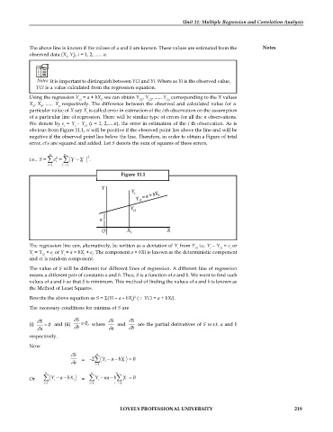
Using the regression Y = a + bX , we can obtain Y , Y , ...... Y corresponding to the X values
Ci i C1 C2 Cn
X , X , ...... X respectively. The difference between the observed and calculated value for a
1 2 n
particular value of X say X is called error in estimation of the i th observation on the assumption
i
of a particular line of regression. There will be similar type of errors for all the n observations.
We denote by e = Y – Y (i = 1, 2,.....n), the error in estimation of the i th observation. As is
i i Ci
obvious from Figure 11.1, ei will be positive if the observed point lies above the line and will be
negative if the observed point lies below the line. Therefore, in order to obtain a Figure of total
error, eis are squared and added. Let S denote the sum of squares of these errors,
n n 2
i 
i.e., S   e  Y  Y Ci  .
2
i
i 1 1 i 
Figure 11.1

The regression line can, alternatively, be written as a deviation of Y from Y i.e. Y – Y = e or
i Ci i Ci i
Y = Y + e or Y = a + bX + e . The component a + bXi is known as the deterministic component
i Ci i i i i
and ei is random component.
The value of S will be different for different lines of regression. A different line of regression
means a different pair of constants a and b. Thus, S is a function of a and b. We want to find such
values of a and b so that S is minimum. This method of finding the values of a and b is known as
the Method of Least Squares.
2
Rewrite the above equation as S = (Yi – a – bX ) ( YCi = a + bXi).
i
The necessary conditions for minima of S are
S¶ S¶ S¶ S¶
(i)  0 and (ii)  0, where and are the partial derivatives of S w.r.t. a and b
a ¶ b ¶ a ¶ b ¶
respectively.
Now
S¶ n

=  2 Y  a bX  0
i
 i
a ¶
i 1
n n n


Or  Y  a bX i  =  Y  na b X  i 0
i
i
i 1 i 1 1 i 
LOVELY PROFESSIONAL UNIVERSITY 219