Page 72 - DECO405_MANAGERIAL_ECONOMICS

Unit 5: Elasticity of Demand

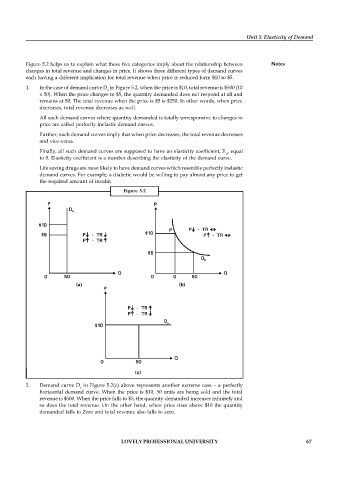
Figure 5.2 helps us to explain what these five categories imply about the relationship between Notes
changes in total revenue and changes in price. It shows three different types of demand curves
each having a different implication for total revenue when price is reduced form $10 to $5.

1. In the case of demand curve D in Figure 5.2, when the price is $10, total revenue is $500 (10
a
x 50). When the price changes to $5, the quantity demanded does not respond at all and
remains at 50. The total revenue when the price is $5 is $250. In other words, when price
decreases, total revenue decreases as well.
All such demand curves where quantity demanded is totally unresponsive to changes in
price are called perfectly inelastic demand curves.
Further, such demand curves imply that when price decreases, the total revenue decreases
and vice-versa.

Finally, all such demand curves are supposed to have an elasticity coefficient, E , equal
d
to 0. Elasticity coefficient is a number describing the elasticity of the demand curve.
Life saving drugs are most likely to have demand curves which resemble perfectly inelastic
demand curves. For example, a diabetic would be willing to pay almost any price to get
the required amount of insulin.
Figure 5.2

2. Demand curve D in Figure 5.2(c) above represents another extreme case – a perfectly
c
horizontal demand curve. When the price is $10, 50 units are being sold and the total
revenue is $500. When the price falls to $5, the quantity demanded increases infinitely and
so does the total revenue. On the other hand, when price rises above $10 the quantity
demanded falls to Zero and total revenue also falls to zero.

LOVELY PROFESSIONAL UNIVERSITY 67