Page 201 - DMGT404 RESEARCH_METHODOLOGY

Unit 9: Correlation and Regression

Remarks: Notes
1. l  0 is a smoothing parameter, controlling the trade-off between fidelity to the data and
roughness of the function estimate.
2. The integral is evaluated over the range of the x .
i
3. As  0 (no smoothing), the smoothing spline converges to the interpolating spline.
4. As  (infinite smoothing), the roughness penalty becomes paramount and the estimate
converges to a linear least-squares estimate.
5. The roughness penalty based on the second derivative is the most common in modern
statistics literature, although the method can easily be adapted to penalties based on other
derivatives.
6. In early literature, with equally-spaced x , second or third-order differences were used in
i
the penalty, rather than derivatives.
7. When the sum-of-squares term is replaced by a log-likelihood, the resulting estimate is
termed penalized likelihood. The smoothing spline is the special case of penalized likelihood
resulting from a Gaussian likelihood.
Multivariate Adaptive Regression Splines (MARS) is a form of regression analysis introduced
by Jerome Friedman in 1991. It is a non-parametric regression technique and can be seen as an
extension of linear models that automatically models non-linearities and interactions.
The term “MARS” is trademarked and licensed to Salford Systems.
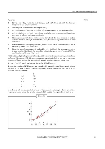
This section introduces MARS using a few examples. We start with a set of data: a matrix of input
variables x, and a vector of the observed responses y, with a response for each row in x. For
example, the data could be:
x y
10.5 16.4
10.7 18.8
10.8 19.7
... ...
20.6 77.0
Here there is only one independent variable, so the x matrix is just a single column. Given these
measurements, we would like to build a model which predicts the expected y for a given x.

Figure 9.8

LOVELY PROFESSIONAL UNIVERSITY 195