Page 274 - DMGT404 RESEARCH_METHODOLOGY

Research Methodology

Notes
ss within = 24 =
(ii) MS within = - 2.67
(n k) 9
where (n – k) is the df.

Step 6: Now we will have to compute F ratio by analysing our samples. The formula for computing
ss between
'F' ratio is:
ss within
4.00
Thus for our example, F ratio = = 1.5
2.67
Step 7: Now we will have to analyze whether various methods of incentives and gain sharing
differ significantly at 5% and 1% 'F' limits. For this, we need to compare observed 'F' ratio with
'F' table values. When observed 'F' value at given degrees of freedom is either equal to or less
than the table value, difference is considered insignificant. In reverse cases, i.e., when calculated
'F' value is higher than table-F value, the difference is considered significant and accordingly we
draw our conclusion.
For example, our observed 'F' ratio at degrees of freedom (v * & v **, i.e., and 9) is 1.5. The table
1 2
value of F at 5% level with df 2 and 9 (v = 2, v = 9) is 4.26. Since the table value is higher than
1 2
the observed value, difference in rate of productivity due to various methods of incentives and
gain sharing is considered insignificant. At 1% level with df 2 and 9, we get the table value of F
as 8.02 and we draw the same conclusion.
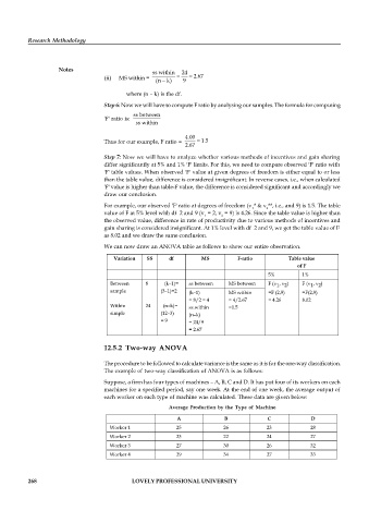
We can now draw an ANOVA table as follows to show our entire observation.

Variation SS df MS F-ratio Table value
of F
5% 1%
Between 8 (k–1)= ss between MS between F (v , v ) F (v , v )
2
2
1
1
sample (3–1)=2 (k–1) MS within =F (2,9) =F(2,9)
= 8/2 = 4 = 4/2.67 = 4.26 8.02
Within 24 (n–k)= ss.within =1.5
simple (12–3) (n–k)
= 9 = 24/9
= 2.67

12.5.2 Two-way ANOVA

The procedure to be followed to calculate variance is the same as it is for the one-way classification.
The example of two-way classification of ANOVA is as follows:
Suppose, a firm has four types of machines – A, B, C and D. It has put four of its workers on each
machines for a specified period, say one week. At the end of one week, the average output of
each worker on each type of machine was calculated. These data are given below:

Average Production by the Type of Machine
A B C D
Worker 1 25 26 23 28
Worker 2 23 22 24 27
Worker 3 27 30 26 32
Worker 4 29 34 27 33

268 LOVELY PROFESSIONAL UNIVERSITY