Page 264 - DCOM504_SECURITY_ANALYSIS_AND_PORTFOLIO_MANAGEMENT

Unit 10: Portfolio Analysis

Notes
Example: Consider a portfolio of two equity shares A and B. The expected return on A is,
say, 15% and that on B is 20%. Further, assume that we have invested 40% of our fund in share A
and the remaining in B. Then, what will be the expected portfolio return?
Solution: The expected portfolio return will be 0.40 × 15 + 0.60 × 20 = 18%.

It may be noted here that portfolio weight can be either positive or negative; in case of securities,
the weight will be negative when investor enters into ‘short sales.’ Usually, investors buy
securities first and sell them later. But with a ‘short sale’ this process is reversed; the investors
sell first the securities that they do not possess, and buy them later to cover the sales. Since
institutional investors in our country do not enter into such sales, we will ignore the situation of
short sales in the present discussion as well as in our dealing with the subject matter in subsequent
units.
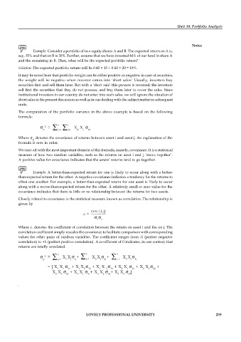
The computation of the portfolio variance in the above example is based on the following
formula:

n n
2 = X X
p i 1 j 1 pi j pj
Where denotes the covariance of returns between asset i and asset j. An explanation of the
pj
formula is now in order.
We start off with the most important element of this formula, namely, covariance. It is a statistical
measure of how two random variables, such as the returns on asset i and j, ‘move together’.
A positive value for covariance indicates that the assets’ returns tend to go together.

Example: A better-than-expected return for one is likely to occur along with a better-
than-expected return for the other. A negative covariance indicates a tendency for the returns to
offset one another. For example, a better-than-expected return for one asset is likely to occur
along with a worse-than-expected return for the other. A relatively small or zero value for the
covariance indicates that there is little or no relationship between the returns for two assets.

Closely related to covariance is the statistical measure known as correlation. The relationship is
given by
cov. (i,j)
c =

i j

Where c. denotes the coefficient of correlation between the return on asset i and the on j. The
correlation coefficient simply rescales the covariance to facilitate comparison with corresponding
values for other pairs of random variables. The coefficient ranges from -1 (perfect negative
correlation) to +1 (perfect positive correlation). A co-efficient of 0 indicates, in our context, that
returns are totally unrelated.
3 3 3
2 = X X + X X + X X
p j 1 1 j ij j 1 2 j 2j j 1 3 j 3j
= [ X X + X X + X X + X X + X X +
1 1 11 1 2 12 1 3 13 2 1 21 2 2 22
X X + X X + X X + X X ]
2 3 23 3 1 31 3 2 32 3 3 33

LOVELY PROFESSIONAL UNIVERSITY 259