Page 49 - DCAP108_DIGITAL_CIRCUITS_AND_LOGIC_DESIGNS

Digital Circuits and Logic Design

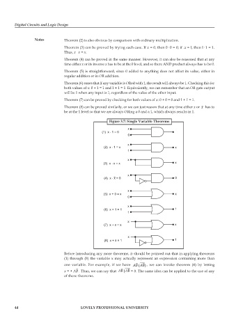
Notes Theorem (2) is also obvious by comparison with ordinary multiplication.
Theorem (3) can be proved by trying each case. If x = 0, then 0· 0 = 0; if .x = l, then l· 1 = 1.
Thus, x x = x.
Theorem (4) can be proved in the same manner. However, it can also be reasoned that at any
time either x or its inverse x has to be at the 0 level, and so there AND product always has to be 0.

Theorem (5) is straightforward, since 0 added to anything does not affect its value, either in
regular addition or in OR addition.
Theorem (6) states that if any variable is ORed with 1, the result will always be 1. Checking this for
both values of x: 0 + 1 = 1 and 1 + 1 = 1. Equivalently, we can remember that an OR gate output
will be 1 when any input is 1, regardless of the value of the other input.

Theorem (7) can be proved by checking for both values of x: 0 + 0 = 0 and 1 + 1 = 1.
Theorem (8) can be proved similarly, or we can just reason that at any time either x or x has to
be at the 1 level so that we are always ORing a 0 and a 1, which always results in 1.

Figure 3.7: Single Variable Theorems
x
(1) x . 1=0
0

x
(2) x . 1=x x
1

x
(3) x . x=x x

x
(4) x . x=0 0

x
(5) x+0=x x
0
x
(6) x+1=1 1
1
x
(7) x+x=x x

x
(8) x+x=1 1

Before introducing any more theorems, it should be pointed out that in applying theorems
(1) through (8) the variable x may actually represent an expression containing more than
one variable. For example, if we have AB AB( ) , we can invoke theorem (4) by letting
x = • AB . Thus, we can say that AB AB( = 0. The same idea can be applied to the use of any
of these theorems.

44 LOVELY PROFESSIONAL UNIVERSITY