Page 200 - DMTH202_BASIC_MATHEMATICS_II

Unit 14: Probability

Notes
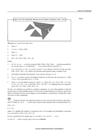
Figure 14.9: The Probability Measure has the Similar Properties as the “Area”

Theorem: Let A and B be events. Then,
1. P() = 0.

2. A  B = ! P(A)  P(B).
3. P(A)  1.
4. P(Ac) = 1 – P(A).
5. P(A  B) = P(A) + P(B) – P(A  B).

Proof:
1.  =     ···, so, by the sum rule, P() = P() + P() + P()+· · · , and consequently, by
the second axiom, 1 = 1+P()+P()+· · · , from which it follows that P() = 0.

2. If A  B, then B = A (B Ac), where A and B Ac are disjoint. Therefore, by the sum rule,
P(B) = P(A) + P(B  Ac), which is (by the first axiom) greater than or equal to P(A).
3. This follows directly from property 2 and axiom 2, because A  .

4.  = A  Ac, where A and Ac are disjoint. Therefore, by the sum rule and axiom 2: 1 = P()
= P(A) + P(Ac), and thus P(Ac) = 1 – P(A).
5. Write A  B as the disjoint union of A and B  Ac. Then, P(A  B) = P(A) + P(B  Ac). Also,
B = (A  B)  (B  Ac), so that P(B) = P(A  B)+ P(B  Ac). Merging these two equations
gives P(A  B) = P(A) + P(B) – P(A  B).

We have now finished our model for a random experiment. It is up to the modeler to state the
sample space  and probability gauge P which most strongly illustrates the definite experiment.
This is not always as clear-cut as it appears, and sometimes it is functional to model only certain
observations in the experiment.

Example: Consider the experiment where we toss a fair die. How should we describe 
and P? Clearly,  = {1, 2, . . . , 6}; and some common sense displays that we should define P by

P(A) = |A|
6, A  ,
where |A| signifies the number of elements in set A. For example, the probability of receiving
an even number is P({2, 4, 6}) = 3/6 = 1/2.
In many applications the sample space is countable, i.e.  = {a1, a2, . . . , an} or
 = {a1, a2, . . .}. Such a sample space is known as discrete.

LOVELY PROFESSIONAL UNIVERSITY 195