Page 221 - DCAP601_SIMULATION_AND_MODELING

Unit 12: Design and Evaluation of Simulation Experiments (II)

Notes
 2
2
  MSE (X ) 
n n
n
Moreover, by the Central Limit Theorem (CLT), X is asymptotically normally distributed as
n
the sample size n increases, i.e.,
n 1/2 [X    N (0, 2 )asn   ,
]
n
where N(a, b) is a normal random variable with mean a and variance b, and  denotes
convergence in distribution.

We thus use this large-sample theory to justify the approximation




N
n
( P X  ) x  P ( ( , 2 / ) x ) P ( (0,1) (x   )/  2 / ) .
N

n
n
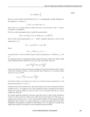
Based on this normal approximation, a (1 — )100% confidence interval for  based on the
sample mean X is
n

[X  z  /2 ( / n X  z  /2 ( / n )]
),

n
n
Where
( P z  N (0,1)  z ) 1   .


 /2  /2
A common choice is a 95% confidence interval, which corresponds to  = 0.05; then z = 1.96
/2
 2.
The statistical precision is typically described by either the absolute width or the relative width
of the confidence interval, denoted by w () and w (), respectively, which are
a r
2z /2  2z /2 

w ( )   and w ( ) 

a r
n  n
There are circumstances where each measure is preferred. For specified absolute width or relative
width of the confidence interval,  and for specified level of precision , the required sample
size n () or n () is then
a r
z
z
4 2 2 4 2 2
n a ( , )   /2 or n r ( , )   /2 (1)




2 2
 2  
2
From these formulas, we see that n (, ) and n (, ) are both inversely proportional to  and
a r
directly proportional to  and z  2 /2.
2
Standard statistical theory describes how observations (data) can be used to estimate the unknown
quantities  and  . We might use a two-stage sampling procedure, exploiting the first stage to
2
estimate the required sample size. However, here we are concerned with what we can do
without any data at all.
We propose applying additional information about the model to obtain rough preliminary
estimates for these parameters without data. Following the general approach of this paper, we
2
suggest trying to estimate  and  before conducting the simulation by analyzing the probability
distribution of the outcome of a single replication, X (using knowledge about the model).
n
Admittedly, this preliminary estimation is often difficult to do; our approach is usually more
useful in the context of one long run, which is discussed in the next section.
LOVELY PROFESSIONAL UNIVERSITY 215