Page 228 - DCAP601_SIMULATION_AND_MODELING

Simulation and Modelling

Notes To describe the rescursive algorithm for BD processes, we start by observing that for a BD
process Poisson’s equation xQ = y is equivalent to the system of equations

x   x (   ) x   y , j  0,

j 1 j 1 j j j j 1 j 1 j
where x = x = 0. Upon adding the first j +1 equations, we obtain the desired recursive
—1 m+1
algorithm,
x  ( x  8 )/ ,

j 1 j j j j 1
where

j
j 
s  y i
i 0
Hence, Poisson’s equation for BD processes can indeed be solved recursively.
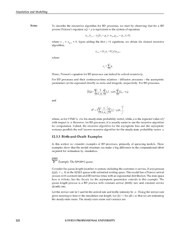
For BD processes and their continuous-time relatives - diffusion processes - the asymptotic
parameters can be expressed directly as sums and integrals, respectively. For BD processes,

m 1 1 j j

 ( )    (f   ) i (   k )
k
i
j 0   j i 0  k 0 
j
and
2
m 1 1  j 
2
  2   (f   ) i  ,
i
j 0   j  i 0 
j
where, as for CTMC’s,  is the steady-state probability vector, while  is the expected value of f
with respect to . However, for BD processes, it is usually easier to use the recursive algorithm
for computation. Indeed, the recursive algorithm for the asymptotic bias and the asymptotic
variance parallels the well known recursive algorithm for the steady-state probability vector .
12.3.3 Birth-and-Death Examples

In this section we consider examples of BD processes, primarily of queueing models. These
examples show that the model structure can make a big difference in the computational effort
required for estimation by simulation.

Example: The M=M=1 queue.

Consider the queue-length (number in system, including the customer in service, if any) process
{Q(t) : t  0} in the M/M/1 queue with unlimited waiting space. This model has a Poisson arrival
process with constant rate and IID service times with an exponential distribution. The state space
here is infinite, but the theory for the asymptotic parameters extends to this example. The
queue-length process is a BD process with constant arrival (birth) rate and constant service
(death) rate.
Let the service rate be 1 and let the arrival rate and traffic intensity be  . Fixing the service rate
gives meaning to time in the simulation run length. Let f(i) = i for all i, so that we are estimating
the steady-state mean. The steady-state mean and variance are

222 LOVELY PROFESSIONAL UNIVERSITY