Page 231 - DCAP601_SIMULATION_AND_MODELING

Unit 12: Design and Evaluation of Simulation Experiments (II)

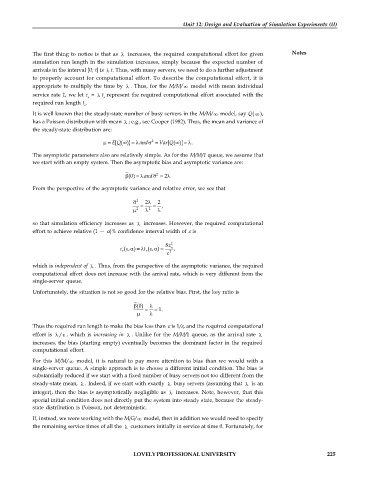
The first thing to notice is that as  increases, the required computational effort for given Notes
simulation run length in the simulation increases, simply because the expected number of
arrivals in the interval [0; t] is  t. Thus, with many servers, we need to do a further adjustment
to properly account for computational effort. To describe the computational effort, it is
appropriate to multiply the time by  . Thus, for the M/M/  model with mean individual
service rate 1, we let c =  t represent the required computational effort associated with the
r r
required run length t .
r
It is well known that the steady-state number of busy servers in the M/M/  model, say Q(  ),
has a Poisson distribution with mean  ; e.g., see Cooper (1982). Thus, the mean and variance of
the steady-state distribution are:

2

Q

Q
  E [ ( )]   and  Var [ ( )]   .
The asymptotic parameters also are relatively simple. As for the M/M/1 queue, we assume that
we start with an empty system. Then the asymptotic bias and asymptotic variance are:
2
 (0)   and  2
From the perspective of the asymptotic variance and relative error, we see that
 2 2 2
  ,
 2  2 

so that simulation efficiency increases as  increases. However, the required computational
effort to achieve relative (1 — )% confidence interval width of  is

8z 2

c ( , )   t ( , )   ,



r r 2

which is independent of  . Thus, from the perspective of the asymptotic variance, the required
computational effort does not increase with the arrival rate, which is very different from the
single-server queue.
Unfortunately, the situation is not so good for the relative bias. First, the key ratio is
 (0) 
  1.
 
Thus the required run length to make the bias less than  is 1/, and the required computational
effort is  / , which is increasing in  . Unlike for the M/M/1 queue, as the arrival rate 
increases, the bias (starting empty) eventually becomes the dominant factor in the required
computational effort.
For this M/M/  model, it is natural to pay more attention to bias than we would with a
single-server queue. A simple approach is to choose a different initial condition. The bias is
substantially reduced if we start with a fixed number of busy servers not too different from the
steady-state mean,  . Indeed, if we start with exactly  busy servers (assuming that  is an
integer), then the bias is asymptotically negligible as  increases. Note, however, that this
special initial condition does not directly put the system into steady state, because the steady-
state distribution is Poisson, not deterministic.
If, instead, we were working with the M/G/  model, then in addition we would need to specify
the remaining service times of all the  customers initially in service at time 0. Fortunately, for

LOVELY PROFESSIONAL UNIVERSITY 225