Page 236 - DCAP601_SIMULATION_AND_MODELING

Simulation and Modelling

Notes Scaling of Time and Space

To obtain relatively simple approximate stochastic processes, we often consider stochastic-
process limits, as in Whitt (2002). (We elaborate below.) To establish appropriate stochastic-
process limits, we usually consider not just one stochastic process but a family of stochastic
processes constructed by scaling time and space. It is thus important to know how the
asymptotic parameters change under such scaling.
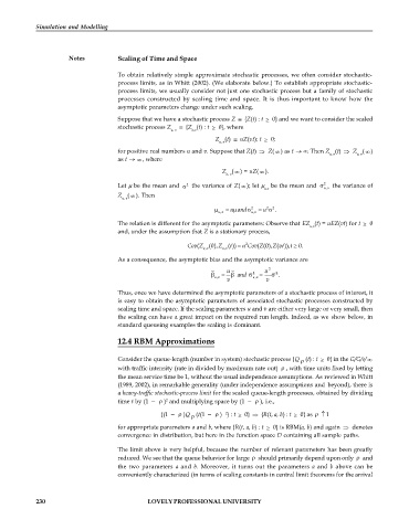
Suppose that we have a stochastic process Z  {Z(t) : t  0} and we want to consider the scaled
stochastic process Z  {Z (t) : t  0}, where
u, v u;v
Z (t)  uZ(vt); t  0;
u, v
for positive real numbers u and v. Suppose that Z(t)  Z(  ) as t  . Then Z (t)  Z (  )
u, v u, v
as t   , where
Z (  ) = uZ(  ).
u, v
Let  be the mean and  the variance of Z(  ); let  be the mean and  2 the variance of
2
u,v , u v
Z (  ). Then
u, v
2

  u and 2  u  2 .
, u v , u v
The relation is different for the asymptotic parameters: Observe that EZ (t) = uEZ(vt) for t  0
u,v
and, under the assumption that Z is a stationary process,
2
Cov (Z (0),Z ( )) u Cov ( (0), ( )),t  0.
vt
t
Z

Z
, u v , u v
As a consequence, the asymptotic bias and the asymptotic variance are
u u 2
   and  2   2 .
, u v , u v
v v
Thus, once we have determined the asymptotic parameters of a stochastic process of interest, it
is easy to obtain the asymptotic parameters of associated stochastic processes constructed by
scaling time and space. If the scaling parameters u and v are either very large or very small, then
the scaling can have a great impact on the required run length. Indeed, as we show below, in
standard queueing examples the scaling is dominant.
12.4 RBM Approximations

Consider the queue-length (number in system) stochastic process {Q (t) : t  0} in the G/G/s/ 

with traffic intensity (rate in divided by maximum rate out)  , with time units fixed by letting
the mean service time be 1, without the usual independence assumptions. As reviewed in Whitt
(1989, 2002), in remarkable generality (under independence assumptions and beyond), there is
a heavy-traffic stochastic-process limit for the scaled queue-length processes, obtained by dividing
time t by (1 —  ) and multiplying space by (1 —  ), i.e.,
2
—2
{(1 —  )Q (t(1 —  ) ) : t  0}  {R(t, a, b) : t  0} as   1

for appropriate parameters a and b, where {R(t, a, b) : t  0} is RBM(a, b) and again  denotes
convergence in distribution, but here in the function space D containing all sample paths.

The limit above is very helpful, because the number of relevant parameters has been greatly
reduced. We see that the queue behavior for large  should primarily depend upon only  and
the two parameters a and b. Moreover, it turns out the parameters a and b above can be
conveniently characterized (in terms of scaling constants in central limit theorems for the arrival

230 LOVELY PROFESSIONAL UNIVERSITY