Page 204 - DECO101_MICRO_ECONOMICS_ENGLISH

Unit 13: Oligopoly

The second order condition for equilibrium requires that Notes

2
∂Π i ∂ 2 R i − ∂ 2 C i
∂ X 2 i = ∂ X 2 i ∂ X 2 i < 0 (i=1,2)
or

∂ 2 R ∂ 2 C
i < i
∂ X 2 ∂ X 2
i i
Each duopolist’s MR must be increasing less rapidly than his MC, that is, the MC must cut the
MR from below, for both duopolists.

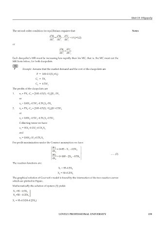
Example: Assume that the market demand and the cost of the duopolists are

P = 100–0.5(X +X )
1 2
C = 5X 1
1
C = 0.5X 2
2 2

The profits of the duopolists are
1. π = PX –C = [100–0.5(X +X )]X –5X 1
1
1
1
1
2
1
or
π = 100X –0.5X –0.5X X –5X
2
1 1 1 1 2 1
2. π = PX –C = [100–0.5(X +X )]X –0.5X 2
2
2
2
2
1
2
2
or
π = 100X –0.5X –0.5X X –0.5X 2
2
2 2 2 1 2 2
Collecting terms we have
π = 95X –0.5X –0.5X X 2
2
1
1
1
1
and
π = 100X –X –0.5X X
2
2 2 2 1 2
For profit maximisation under the Cournot assumption we have

⎧ ∂Π 1 ⎫
−
⎪ = 0=95 X − 0.5X 2 ⎪
1
⎪ ∂ X 2 ⎪
⎨ ∂Π ⎬ ...... (3)
⎪ 2 = 0=100 2X − 0.5X ⎪
−
⎪ ∂ X 2 2 1 ⎪ ⎭
⎩
The reaction functions are:
X = 95–0.5X 2
1
X = 50–0.25X
2 1
The graphical solution of Cournot’s model is found by the intersection of the two reaction curves
which are plotted in Figure.
Mathematically the solution of system (3) yields
−
X =95 0.5X 2 ⎤
1
−
X =50 0.25X 1⎦ ⎥
2
X = 95–0.5(50–0.25X )
1
1
LOVELY PROFESSIONAL UNIVERSITY 199