Page 216 - DECO101_MICRO_ECONOMICS_ENGLISH
P. 216

Unit 13: Oligopoly


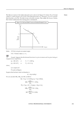
          The full cost version of the kinked demand curve is shown by Figure 13.6 where ON  is Normal   Notes
                                                                              1
          output, P  is full cost price and A P B  is the kinked demand curve. Elasticity e  for AP  is greater
                                                                        1
                  1
                                                                              1
                                    1
                                      1
                                       1
          than elasticity e  for P B . The kink occurs at the full cost price. Thus unlike the Sweezy version,
                             1
                           1
                       1
          this version explains how the existing price is determined.
                          Figure 13.6: Hall and Hitch Version of Kinked Demand Curve
                             Price  A 1    e 1


                           Full P 1                P 1
                           cost                        e 2
                          price


                              0                  N 1      B 1     Output

          Notes: OP  Full cost price at normal output
                    1
                 ON  = Normal output, e  > e
                    1                1  2

                 Example: Suppose that the demand functions for price increases and for price facing an
          oligopolist are, respectively,
                 Q  = 280–40 P     or   P  = 7 – 0.025 Q
                   1        1           1          1
                 Q  = 100–10 P     or   P  = 10–0.1 Q
                   2        2           2        2
          where,
                 Q is output and
                 P is price in Rupees.


          Suppose that the firm’s total cost function is
                                         TC = 2Q+0.025Q 2
          We can calculate MR , MR , and MC as follows
                           1   2
                               TR  = P Q  = (7–0.025Q ) Q  = 7Q –0.025Q
                                                                2
                                  1
                                                                 1
                                                  1
                                                     1
                                       1
                                                         1
                                     1
                                            d(TR )
                                      MR =      1  =7 0.05Q 1
                                                    −
                                         1
                                             dQ 1
                                TR  = P Q  = (10 – 0.1Q )Q  = 10Q –0.1Q
                                                                2
                                  2   2  2        2  2    2     2
                                           d(TR )
                                      MR =      2  =10 0.2Q 2
                                                    -
                                         2
                                             dQ  2
                                            d(TC)
                                       MC=       =2 0.05Q
                                                   +
                                            d(Q)
                                           LOVELY PROFESSIONAL UNIVERSITY                                   211
   211   212   213   214   215   216   217   218   219   220   221