Page 240 - DCOM203_DMGT204_QUANTITATIVE_TECHNIQUES_I

Unit 11: Analysis of Time Series

Solution. Notes
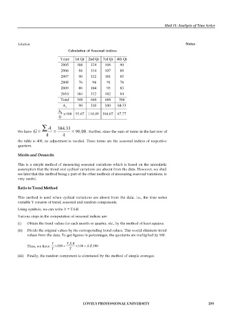
Calculation of Seasonal Indices
Years 1st Qr 2nd Qr 3rd Qr 4th Qr
2005 106 124 104 90
2006 84 114 107 88
2007 90 112 101 85
2008 76 94 91 76
2009 80 104 95 83
2010 104 112 102 84
Total 540 660 600 506
A i 90 110 100 84.33
A i 100 93.67 114.49 104.07 87.77
G

A 384.33
We have G i 96.08 . Further, since the sum of terms in the last row of
4 4
the table is 400, no adjustment is needed. These terms are the seasonal indices of respective
quarters.

Merits and Demerits

This is a simple method of measuring seasonal variations which is based on the unrealistic
assumption that the trend and cyclical variations are absent from the data. However, we shall
see later that this method being a part of the other methods of measuring seasonal variations, is
very useful.

Ratio to Trend Method

This method is used when cyclical variations are absent from the data, i.e., the time series
variable Y consists of trend, seasonal and random components.
Using symbols, we can write Y = T.S.R
Various steps in the computation of seasonal indices are:

(i) Obtain the trend values for each month or quarter, etc., by the method of least squares.
(ii) Divide the original values by the corresponding trend values. This would eliminate trend
values from the data. To get figures in percentages, the quotients are multiplied by 100.

S
Y T . .R
R
Thus, we have 100 100 S . .100
T T
(iii) Finally, the random component is eliminated by the method of simple averages.

LOVELY PROFESSIONAL UNIVERSITY 235