Page 234 - DMGT209_QUANTITATIVE_TECHNIQUES_II

Unit 11: Multiple Regression and Correlation Analysis

Note: Notes

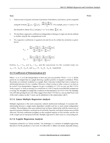
1. Various sums of squares and sums of products of deviations, used above, can be computed
 X  X 
using the formula  x x  X X  p q . For example, put p = 1 and q = 2 in
p q 
q
p
n
the formula to obtain X X and put p = q = 2, to obtain  x 2 2 , etc.
1 2
2. The fact that a regression coefficient is independent of change of origin can also be utilised
to further simplify the computational work.
3. The regression coefficients of equations (2) and (3) can be written by symmetry as given
below:

 x x 1  x  x x 3  x x 
2
 
2
1 3
2
3
b = 2 2 2
 
21.3  x 1  x  x x 
1 3
3
 x x 3  x  x x 1  x x 
2
 
1
2
2
1 3
b = 2 2 2
 
23.1  x 1  x  x x 
3
1 3
Further, b = b and b = b and the expressions for the constant terms are
31.2 13.2 32.1 23.1
a  X  b X  b X and a  X  b X  b X respectively.
2.13 2 21.3 1 23.1 3 3.12 3 31.2 1 32.1 2
11.3 Coefficient of Determination ( )
2
When = 1; or -1; or 0, the interpretation of does not pose any problem. When = 1; or –1, all the
points lie on straight line in a graph showing a perfect positive or negative correlation. When
the points are extremely scattered on a graph, then it becomes evident that there is almost no
relationship between the two variables. However, when it comes to other values of, we have to
be careful in its interpretation. Suppose we get a correlation of = 0.9, we may say that = 0.9 is
‘twice as good’ or ‘twice as strong’ as a correlation of = 0.45. It may be noted that this comparison
is wrong. The strength of is judged by coefficient of determination, for = 0.9, = 0.81. We multiply
it by 100, thus getting 81 per cent. Thus suggest that when = 0.9 then we can say that 81 per cent
of the total variation in the Y series can be attributed to the relationship with X.
11.3.1 Linear Multiple Regression Analysis
Multiple regressions is the most commonly utilized multivariate technique. It examines the
relationship between a single metric dependent variable and two or more metric independent
variables. The technique relies upon determining the linear relationship with the lowest sum of
squared variances; therefore, assumptions of normality, linearity, and equal variance are carefully
observed. The beta coefficients (weights) are the marginal impacts of each variable, and the size
of the weight can be interpreted directly. Multiple regression is often used as a forecasting tool.

11.3.2 Logistic Regression Analysis

Sometimes referred to as “choice models,” this technique is a variation of multiple regressions
that allows for the prediction of an event. It is allowable to utilize non-metric (typically binary)

LOVELY PROFESSIONAL UNIVERSITY 229