Page 193 - DMGT404 RESEARCH_METHODOLOGY
P. 193
Unit 9: Correlation and Regression
bivariate data, there will always be two lines of regression. It will be shown later that these two Notes
lines are different, i.e., one cannot be derived from the other by mere transfer of terms, because
the derivation of each line is dependent on a different set of assumptions.
Line of Regression of Y on X
The general form of the line of regression of Y on X is Y = a + bX , where Y denotes the average
Ci i Ci
or predicted or calculated value of Y for a given value of X = X . This line has two constants, a and
i
b. The constant a is defined as the average value of Y when X = 0. Geometrically, it is the intercept
of the line on Y-axis. Further, the constant b, gives the average rate of change of Y per unit change
in X, is known as the regression coefficient.
The above line is known if the values of a and b are known. These values are estimated from the
observed data (X , Y ), i = 1, 2, ...... n.
i i
Notes It is important to distinguish between Y and Y . Where as Y is the observed value,
Ci i i
Y is a value calculated from the regression equation.
Ci
Using the regression YC = a + bX , we can obtain Y , Y , ...... Y corresponding to the X values
i i C1 C2 Cn
X , X , ...... X respectively. The difference between the observed and calculated value for a
1 2 n
particular value of X say Xi is called error in estimation of the i th observation on the assumption
of a particular line of regression. There will be similar type of errors for all the n observations.
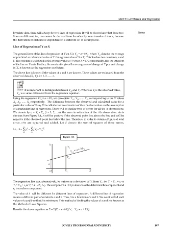
We denote by e = Y – Y (i = 1, 2,.....n), the error in estimation of the i th observation. As is
i i Ci
obvious from Figure 9.4, ei will be positive if the observed point lies above the line and will be
negative if the observed point lies below the line. Therefore, in order to obtain a Figure of total
error, ei¢s are squared and added. Let S denote the sum of squares of these errors,
n
i.e., S = å e = n (Y - Y ) .
i å
2
2
i= 1 i= 1 i Ci
Figure 9.4
Y
Y
Y a bX i
i
+
=
ci
Y
ci
a
O X i X
The regression line can, alternatively, be written as a deviation of Y from Y i.e. Y – Y = e or
i Ci i Ci i
Y = Y + e or Y = a + bX + e . The component a + bX is known as the deterministic component and
i Ci i i i i i
e is random component.
i
The value of S will be different for different lines of regression. A different line of regression
means a different pair of constants a and b. Thus, S is a function of a and b. We want to find such
values of a and b so that S is minimum. This method of finding the values of a and b is known as
the Method of Least Squares.
2
Rewrite the above equation as S = S(Y – a – bX ) (Y = a + bX ).
i i Ci i
LOVELY PROFESSIONAL UNIVERSITY 187

