Page 168 - DMGT501_OPERATIONS_MANAGEMENT

Operations Management

Notes (iv) m = D/n where m = fraction defective
(v) Find n p, n p … n p
1 2 k
(vi) For p < 0.10
Use control limits from respective statistical table else (p >= 0.10)

Calculate control limits by

np ± 3 n.p.q where q = (1– p)
(vii) Test for homogenecity as in (a) for uniform size.
(viii) Accept the ‘p’ of the homogenecity data as the standard of capability of the
process.

Calculation of Process Capability Variable Data

A variable data has two parameters, central tendency and dispersion. Whereas the central
tendency can be corrected easily, its very difficult to examine the dispersion and hence is critical
for assessing the Process Capability.

Range

1. Let us take number of samples k = 25
2. Let us have n = number of observations in each sample = 4 or 5 (uniform)
3. Let R , R … R be the ‘Range’ of sample 1, 2 … k respectively.
1 2 k
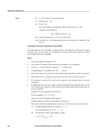
4. Average Range R = summation (R + R + … + R )/k
1 2 k
5. Read off the values of D and D from the statistical table against the sample size selected.
3 4
6. Then UCL & LCL i.e., Upper & Lower Control Limits are given by D . R and D . R
4 3
7. If no reading is outside the Control Limit, accept R as the standard index of process
variability.
8. If readings are beyond Control Limits, reject them and find the revised limits and so on till
the homogenecity is achieved. In this case the revised Rbar shall be the standard index of
process variability.
Calculate Process Capability by the formula

Process Capability = 6 = 6 × R / d
2
where d is from the statistical table against ‘n’.
2
Variation between samples or the stability of the process.
This can be checked by examining the consistency of the sample means as given below:

(a) Calculate sample means of all samples 1, 2, … k.
Let the sample means be X ,X , ........ X .
2
k
1
(b) Calculate the average of the sample averages
X X ........ X
= X 1 2 k
k

162 LOVELY PROFESSIONAL UNIVERSITY