Page 31 - DCOM303_DMGT504_OPERATION_RESEARCH
P. 31
Operations Research
Notes 2.6 Graphical Solutions under Linear Programming
Linear programming problems with two variables can be represented and solved graphically
with ease. Though in real-life, the two variable problems are practiced very little, the interpretation
of this method will help to understand the simplex method.
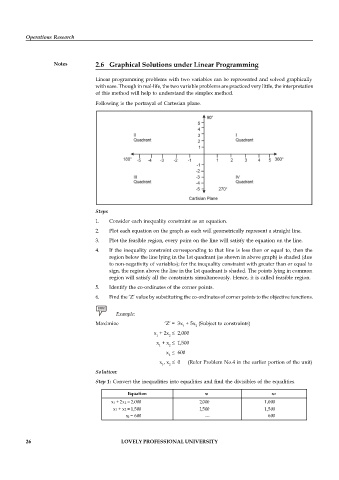
Following is the portrayal of Cartesian plane.
Steps
1. Consider each inequality constraint as an equation.
2. Plot each equation on the graph as each will geometrically represent a straight line.
3. Plot the feasible region, every point on the line will satisfy the equation on the line.
4. If the inequality constraint corresponding to that line is less than or equal to, then the
region below the line lying in the 1st quadrant (as shown in above graph) is shaded (due
to non-negativity of variables); for the inequality constraint with greater than or equal to
sign, the region above the line in the 1st quadrant is shaded. The points lying in common
region will satisfy all the constraints simultaneously. Hence, it is called feasible region.
5. Identify the co-ordinates of the corner points.
6. Find the ‘Z’ value by substituting the co-ordinates of corner points to the objective functions.
Example:
Maximize ‘Z’ = 3x + 5x (Subject to constraints)
1 2
x + 2x 2,000
1 2
x + x 1,500
1 2
x 600
2
x , x 0 (Refer Problem No.4 in the earlier portion of the unit)
1 2
Solution:
Step 1: Convert the inequalities into equalities and find the divisibles of the equalities.
Equation x1 x2
x 1 + 2x 2 = 2,000 2,000 1,000
x1 + x2 = 1,500 1,500 1,500
x 2 = 600 --- 600
26 LOVELY PROFESSIONAL UNIVERSITY

