Page 217 - DECO401_MICROECONOMIC_THEORY_ENGLISH

Microeconomic Theory

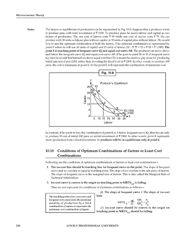
Notes The factors or equilibrium of production can be represented by Fig. 10.8. Suppose that a producer wants
to produce pens with total investment of 1500. To produce pens, he needs labour and capital as two
factors of production. The one unit of labour costs 50 while one unit of capital costs 75. He can
produce with 30 units so labour plus without capital or 20 units of capital plus without labour. He would
love to mix the optimum combination of both the factors. This optimum combination is represented by
point E when he will use 10 units of capital and 15 units of labour (10 × 75 + 15 × 50 = 1,500). The
point E is touching point of Isoquant curve IQ and equal cost curve AB. The producer can move above
and below the Isoquant curve IQ and equal cost curve AB. If he goes to point M or N of Isoquant curve
IQ, then he would find himself on above equal cost line CD, it means he needs to pay more for producing
initial amount of pen (100) rather than investing the fixed level of 1500. In other words, to produce 100
pens, the cost is minimum at point E. So the point E will represent the combination of minimum cost.

Fig. 10.8

Y
Producer's Equilibrium
C
25 IQ
IQ 1 M
20 A
R
Capital 15 E
10
N
5 IQ (100)
S
IQ (100)
1
0 B D X
5 10 15 20 25 3035
Labour

In contrast, if he wants to buy the combination of point R or S below Isoquant curve IQ then he can only
1
to produce 50 out of initial 100 pens on initial investment of 1500. In other words, point E represents
more production from a fixed investment. So producer will be in equilibrium only at point E.

10.10 Conditions of Optimum Combinations of Factors or Least Cost
Combinations

Following are the conditions of optimum combinations of factors or least cost combinations—
1. The iso-cost line should be touching line for Isoquant curve on flat point. The slope of Isoquant
curve and iso-cost line is equal at touching point. The slope of iso-cost line is the rate price of factors.
The slope of Isoquant curve is the marginal rate of factors. This is also called the Marginal Rate of
Technical Substitution.
2. iso-cost curve is convex to the origin on touching point or MRTS is falling.
LK
Thus we can represent the conditions of Optimum combinations as follows—
(i) The slope of Isoquant curve = The slope of iso-cost
The touching point of iso-cost curve and Line
MP
P
Isoquant curve represents the maximum ∆K _____ ___
___
L
L

quantity of production by a fixed MRTS = ∆L = MP =
P
LK
K
K
combination of inputs or represents the (ii) iso-cost curve should be convex to the origin on
minimum cost combination of inputs.
touching point or MRTS should be falling.
LK
210 LOVELY PROFESSIONAL UNIVERSITY