Page 174 - DECO503_INTERNATIONAL_TRADE_AND_FINANCE_ENGLISH

International Trade and Finance

Notes
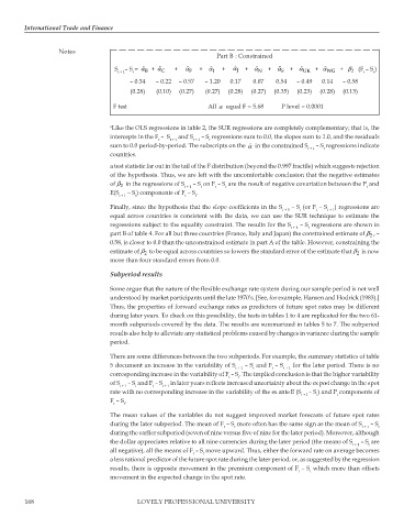
Part B : Constrained
S – S = α ˆ + α ˆ + α ˆ + α ˆ + α ˆ + α ˆ + α ˆ + α ˆ + α ˆ + β (F – S )
J
t + 1 t B C F I N S UK WG 2 t t
– 0.34 – 0.22 – 0.57 – 1.20 0.17 0.07 0.54 – 0.49 0.14 – 0.58
(0.28) (0.10) (0.27) (0.27) (0.28) (0.27) (0.35) (0.23) (0.28) (0.13)

F test All α equal F = 5.68 P level = 0.0001

a Like the OLS regressions in table 2, the SUR regressions are completely complementary; that is, the
intercepts in the F – S and S – S regressions sum to 0.0, the slopes sum to 1.0, and the residuals
t t + 1 t + 1 t
sum to 0.0 period-by-period. The subscripts on the α ˆ in the constrained S – S regressions indicate
t + 1 t
countries.
a test statistic far out in the tail of the F distribution (beyond the 0.997 fractile) which suggests rejection
of the hypothesis. Thus, we are left with the uncomfortable conclusion that the negative estimates
of β in the regressions of S t + 1 – S on F – S are the result of negative covariation between the P and
2
t
t
t
t
E(S – S ) components of F – S .
t + 1 t t t
Finally, since the hypothesis that the slope coefficients in the S – S (or F – S ) regressions are
t + 1 t t t + 1
equal across countries is consistent with the data, we can use the SUR technique to estimate the
regressions subject to the equality constraint. The results for the S – S regressions are shown in
t + 1 t
part B of table 4. For all but three countries (France, Italy and Japan) the constrained estimate of β , –
2
0.58, is closer to 0.0 than the unconstrained estimate in part A of the table. However, constraining the
estimate of β to be equal across countries so lowers the standard error of the estimate that β is now
2
2
more than four standard errors from 0.0.
Subperiod results
Some argue that the nature of the flexible exchange rate system during our sample period is not well
understood by market participants until the late 1970’s. [See, for example, Hansen and Hodrick (1983).]
Thus, the properties of forward exchange rates as predictors of future spot rates may be different
during later years. To check on this possibility, the tests in tables 1 to 4 are replicated for the two 61-
month subperiods covered by the data. The results are summarized in tables 5 to 7. The subperiod
results also help to alleviate any statistical problems caused by changes in variance during the sample
period.

There are some differences between the two subperiods. For example, the summary statistics of table
5 document an increase in the variability of S – S and F – S for the later period. There is no
t + 1 t t t + 1
corresponding increase in the variability of F – S . The implied conclusion is that the higher variability
t t
of S – S and F – S in later years reflects increased uncertainty about the ex post change in the spot
t + 1 t t t + 1
rate with no corresponding increase in the variability of the ex ante E (S – S ) and P components of
t + 1 t t
F – S .
t t
The mean values of the variables do not suggest improved market forecasts of future spot rates
during the later subperiod. The mean of F – S more often has the same sign as the mean of S – S
t t t + 1 t
during the earlier subperiod (seven of nine versus five of nine for the later period). Moreover, although
the dollar appreciates relative to all nine currencies during the later period (the means of S – S are
t + 1 t
all negative), all the means of F – S move upward. Thus, either the forward rate on average becomes
t t
a less rational predictor of the future spot rate during the later period, or, as suggested by the regression
results, there is opposite movement in the premium component of F – S which more than offsets
t t
movement in the expected change in the spot rate.

168 LOVELY PROFESSIONAL UNIVERSITY