Page 78 - DECO503_INTERNATIONAL_TRADE_AND_FINANCE_ENGLISH

International Trade and Finance

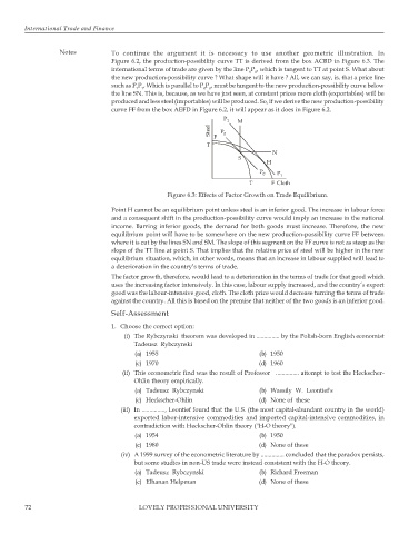
Notes To continue the argument it is necessary to use another geometric illustration. In
Figure 6.2, the production-possibility curve TT is derived from the box ACBD in Figure 6.3. The
international terms of trade are given by the line P P , which is tangent to TT at point S. What about
0 0
the new production-possibility curve ? What shape will it have ? All, we can say, is, that a price line
such as P P , Which is parallel to P P , must be tangent to the new production-possibility curve below
0
0
1
1
the line SN. This is, because, as we have just seen, at constant prices more cloth (exportables) will be
produced and less steel (importables) will be produced. So, if we derive the new production-possibility
curve FF from the box AEFD in Figure 6.2, it will appear as it does in Figure 6.2.
P 1 M
Steel F P 0
T
N
S
H
P 0 P 1

T F Cloth
Figure 6.3: Effects of Factor Growth on Trade Equilibrium.
Point H cannot be an equilibrium point unless steel is an inferior good. The increase in labour force
and a consequent shift in the production-possibility curve would imply an increase in the national
income. Barring inferior goods, the demand for both goods must increase. Therefore, the new
equilibrium point will have to be somewhere on the new production-possibility curve FF between
where it is cut by the lines SN and SM. The slope of this segment on the FF curve is not as steep as the
slope of the TT line at point S. That implies that the relative price of steel will be higher in the new
equilibrium situation, which, in other words, means that an increase in labour supplied will lead to
a deterioration in the country’s terms of trade.
The factor growth, therefore, would lead to a deterioration in the terms of trade for that good which
uses the increasing factor intensively. In this case, labour supply increased, and the country’s export
good was the labour-intensive good, cloth. The cloth price would decrease turning the terms of trade
against the country. All this is based on the premise that neither of the two goods is an inferior good.
Self-Assessment
1. Choose the correct option:
(i) The Rybczynski theorem was developed in ............... by the Polish-born English economist
Tadeusz Rybczynski
(a) 1955 (b) 1950
(c) 1970 (d) 1960
(ii) This econometric find was the result of Professor ............... attempt to test the Heckscher-
Ohlin theory empirically.
(a) Tadeusz Rybczynski (b) Wassily W. Leontief's
(c) Heckscher-Ohlin (d) None of these
(iii) In ..............., Leontief found that the U.S. (the most capital-abundant country in the world)
exported labor-intensive commodities and imported capital-intensive commodities, in
contradiction with Heckscher-Ohlin theory ("H-O theory").
(a) 1954 (b) 1950
(c) 1980 (d) None of these
(iv) A 1999 survey of the econometric literature by ............... concluded that the paradox persists,
but some studies in non-US trade were instead consistent with the H-O theory.
(a) Tadeusz Rybczynski (b) Richard Freeman
(c) Elhanan Helpman (d) None of these

72 LOVELY PROFESSIONAL UNIVERSITY