Page 141 - DECO504_STATISTICAL_METHODS_IN_ECONOMICS_ENGLISH

Unit 9: Correlation: Definition, Types and its Application for Economists

Notes
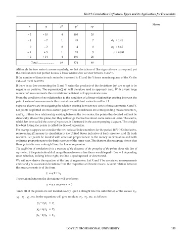
x y x 2 y 2 xy

– 2 – 10 4 100 20

– 1 – 7 1 49 7 σ 1 = 1.41
0 – 2 0 4 0 σ 2 = 8.65

+ 1 + 5 1 25 5 r = 0.981
+ 2 + 14 4 196 28

Total ...................... 10 374 60

Although the two series increase regularly, so that deviations of like signs always correspond, yet
the correlation is not perfect because a linear relation does not exist between X and Y.
If the number of items in each series be increased to 11 and the Y items remain squares of the X’s the
value of r will be 0.974.
If there be no law connecting the X and Y series the products of the deviations (xy) are as apt to be
negative as positive. The expression ∑xy will therefore tend to approach zero. With a very large
number of measurements the correlation coefficient will approximate zero.
From the condition of no relationship to the condition of a linear relationship existing between the
pair of series of measurements the correlation coefficient varies from 0 to ± 1.
Suppose that we are investigating the relation existing between two series of measurements X and Y.
Let points be plotted on cross-section paper whose coordinates are corresponding measurements X
1
and Y . If there be a relationship existing between the two series, the points thus located will not lie
1
chaotically all over the plane, but they will range themselves about some curve or locus. This curve,
which has been called the curve of regression, is illustrated in the accompanying diagram. The straight
line best fitting the points is called the line of regression.
For example suppose we consider the two series of index numbers for the period 1879-1904 inclusive,
representing (1) money in circulation in the United States inclusive of bank reserves, and (2) bank
reserves. Let points be located with abscissas proportionate to the money in circulation and with
ordinates proportionate to the bank reserves of the same year. The chart on the next page shows that
these points lie near a straight line, the line of regression.
The coefficient of correlation (r) is a measure of the closeness of the grouping of the points about this line of
regression. If the points should all range themselves on a line then r would equal + 1 or — 1 depending
upon whether, looking left to right, the line sloped upward or downward.
We will now derive the equation of the line of regression. Let X and Y be associated measurements
and x and y be associated deviations from the respective arithmetic means. A linear relation between
the measurements is of the form
a
Y= 1 X + b 1
The relation between the deviations will be of form
y = ax or –y ax = 0
1
1
Since all of the points are not located exactly upon a straight line the substitution of the values 1 ,
x
v
v
y
x
y 1 , 2 , 2 , etc. in the equations will give residues 1 , 2 , etc. as follows:
y 1 – ax v
1 1 = 1
y 2 – ax v
1 2 = 2
y n – ax v
1 n = n

LOVELY PROFESSIONAL UNIVERSITY 135