Page 146 - DECO504_STATISTICAL_METHODS_IN_ECONOMICS_ENGLISH

Statistical Methods in Economics

Notes 2
(
δ ' = ∑ d m ) '– ' d ;
n

and the coefficient of correlation is
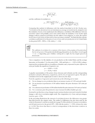
∑ ( ) – ( dd d ) '– ' d ∑dd '–nd d '
ρ = m m = m m
n δδ ' ( 2 –nd m 2 ) ∑ ( d d '2 – nd ' m 2 ) ∑

Comparing this method of differences with the method described in (1) Mr. Hooker says,
“Correlation of the deviations from an instantaneous average (or trend) may be adopted to test
the similarity of more or less marked periodic influences, correlation of the difference between
successive values will probably prove most useful where the similarity of the shorter rapid
changes (with no apparent periodicity) are the subject of investigation, or where the normal
level of one or both series of observations does not remain constant.” He finds that the ordinary
correlation coefficient (r) for the price of corn in Iowa and total production in the United States
for the period 1870 – 1899 is – 0.28, while ρ = – 0.84.

The coefficient of correlation (r) is a measure of the closeness of the grouping of the points about
this line of regression. If the points should all range themselves on a line then r would equal
+ 1 or — 1 depending upon whether, looking left to right, the line sloped upward or
downward.

I have computed ρ for the statistics of corn production in the United States and the average
farm price on December 1* for the period 1866 – 1906 and finds ρ = – 0.833 ± 0.034. Letting x
represent the production difference in millions of bushels, and y represent the price difference in
cents per bushel, the equations of regression are
y = – 0.0256 x + 1.132
x = – 27.05 y + 46.42
A graphic representation of the points whose abscissas and ordinates are the corresponding
production and price differences, respectively, and the line of regression is given. The lack of
correlation between the original pair of series is shown by the chart.
From the equations of regression such statements as the following can be made:
(i) For no change in corn production there is an increase in price of 1.132 cents per bushel.
(ii) For an increase in production of 100 million bushels the price decreases 1.43 cents per
bushel.
(iii) For a decrease in production of 100 million bushels the price increases 3.69 cents per bushel.
(iv) For a stationary price the production must increase 46 million bushels per year.
It seemed to me that if percentage changes in price and production were used instead of absolute
changes a still closer correlation might result. The computation of ρ from such percentages,
however, gave – 0.794.
In the preceding illustrations the amount of correlation between the differences was greater
than that between the original series. The method of differences has also been used by the
writer for Kemmerer’s statistics (considered on page 15 of this article) of (1) money in circulation,
and (2) bank reserves for the period 1879 – 1904 with the result ρ = + 0.392, whereas the value
of r is 0.98. This shows that there is a lack of correspondence of the short-time variations in
these two series.

140 LOVELY PROFESSIONAL UNIVERSITY